
Improving Blind Docking in DOCK6 through an Automated Preliminary Fragment Probing Strategy


Abstract
1. Introduction
2. Methods
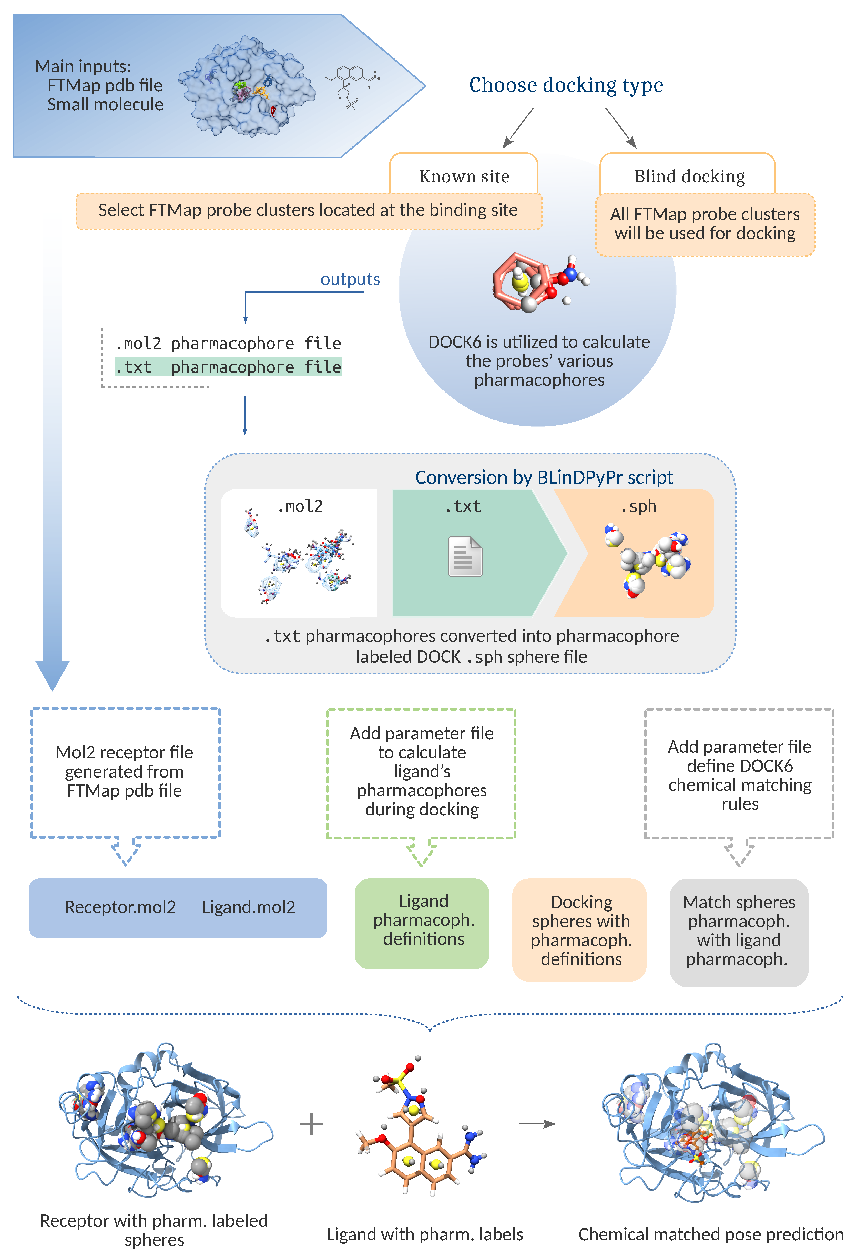
2.1. Pipeline Components
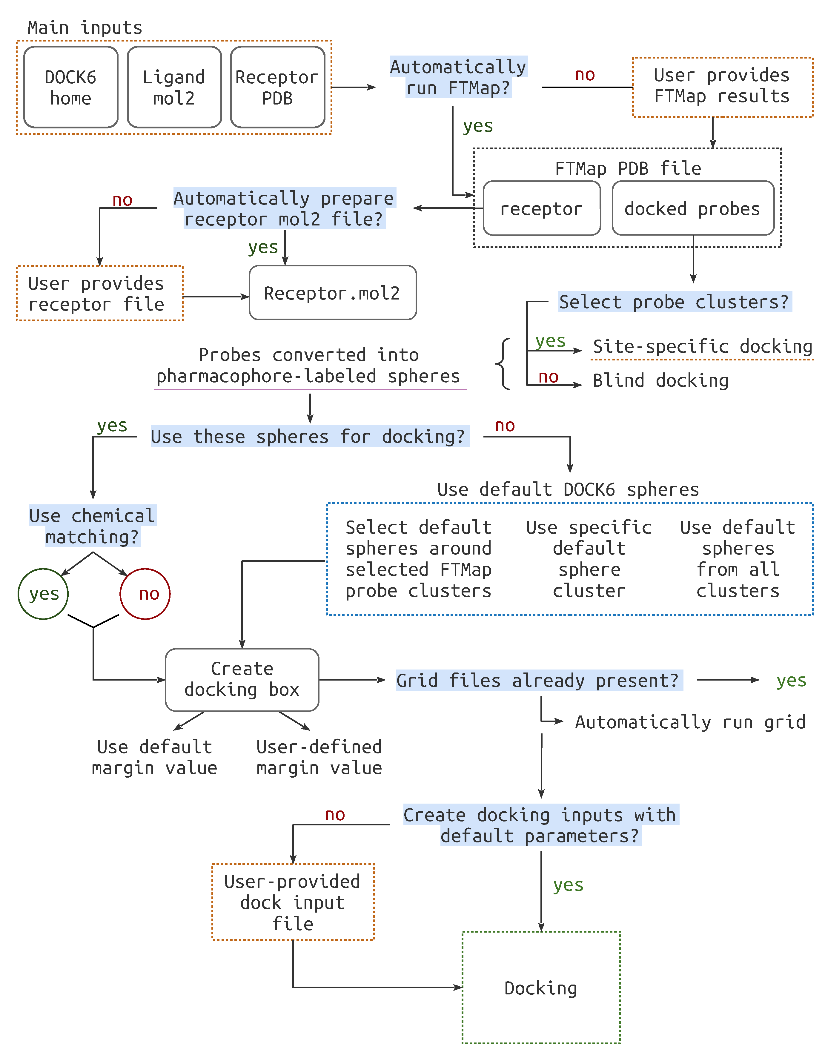
2.2. Pipeline Workflow
2.2.1. File Preparation
2.2.2. Cavity Definition
- FTMap Derived Spheres
- Classic Spheres
2.2.3. Docking Preparation
2.2.4. Docking Run
2.3. Benchmarking
2.3.1. PDBbind Core Set
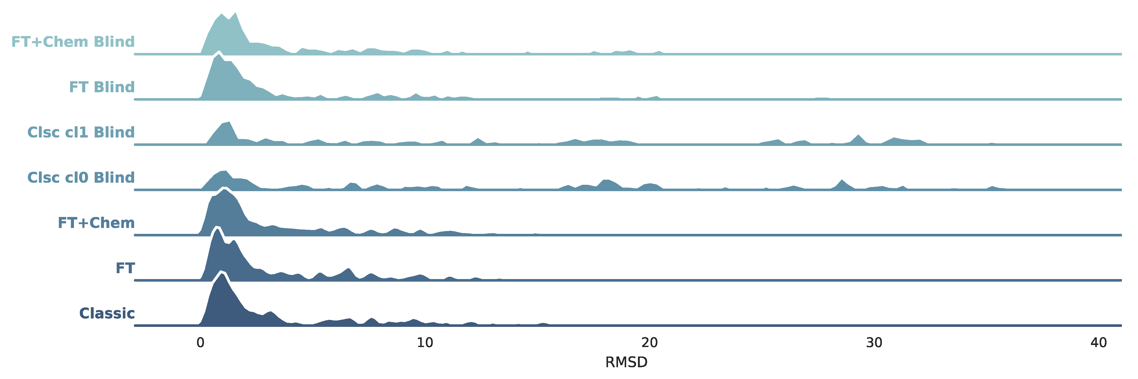
- FT+Chem: Docking is performed on spheres derived from FTMap probe crossclusters, with chemical matching to further orient the ligands. This method was employed for blind and site-specific docking.
- FT: Docking is performed on spheres derived from FTMap probe crossclusters; however, chemical matching is turned off and the spheres pharmacophore labels do not influence pose prediction. This method was employed for blind and site-specific docking.
- Manual site-specific: It is a classic DOCK6 site-specific docking run. The accessory tool sphgen is used to generate classic spheres from a receptor surface file. DOCK6 sphere selector is then employed to select those in a radius of three Angstroms around the selected probe crossclusters,
- Cavity-detection guided (Cluster 1): It is a classic DOCK6 run using the first sphere cluster, defined by sphgen as the most likely to overlap with the real binding site.
- Blind: It is a classic DOCK6 blind run using all the generated spheres (sphere Cluster 0). This is the only case where DOCK6 must evaluate docking poses throughout the whole protein surface.
2.3.2. Astex Diverse Set
- FT+Chem Blind
- FT Blind
- Cavity-detection Blind (Cluster 1)
3. Results and Discussion
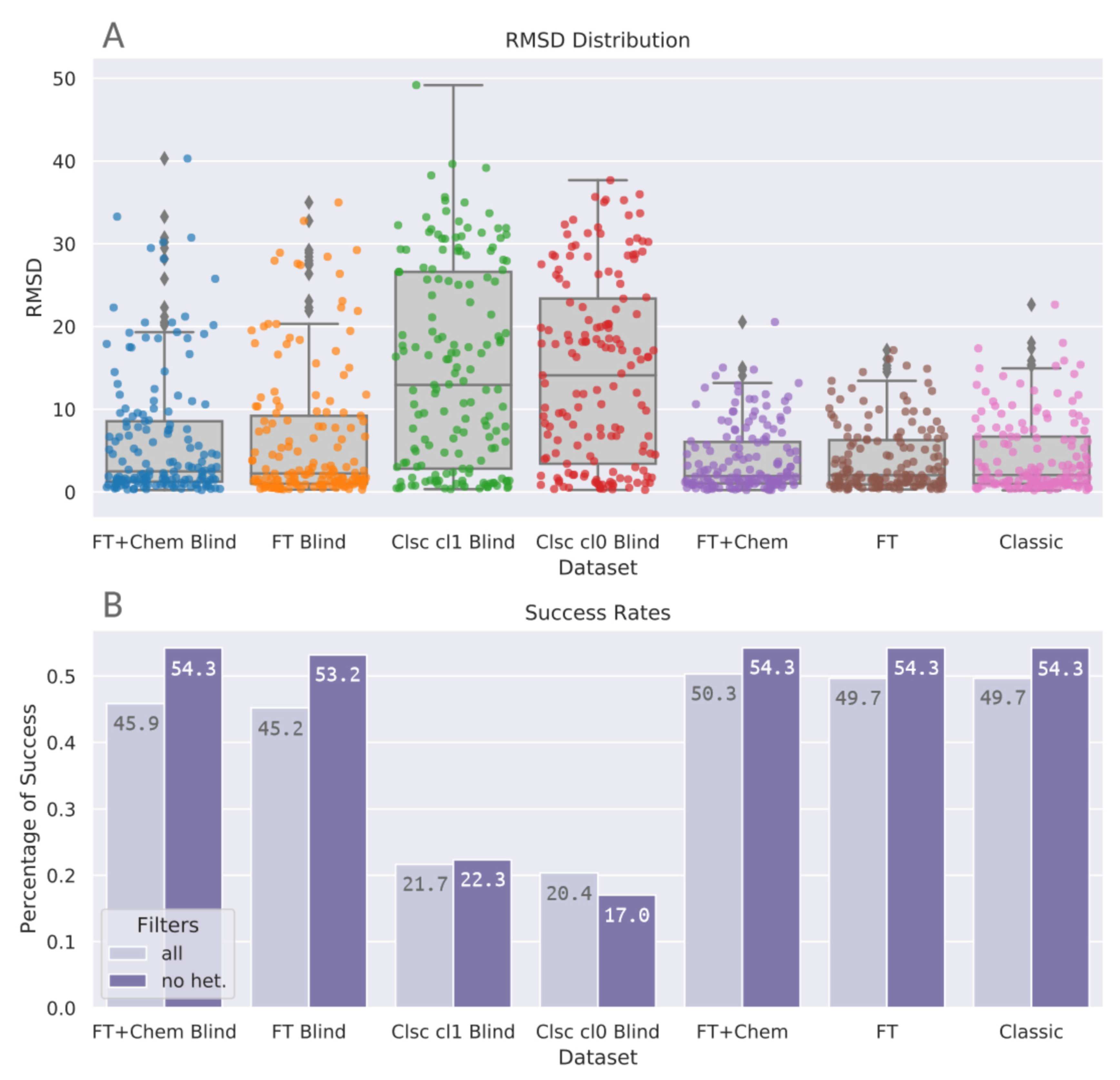
3.1. PDBbind Core Set
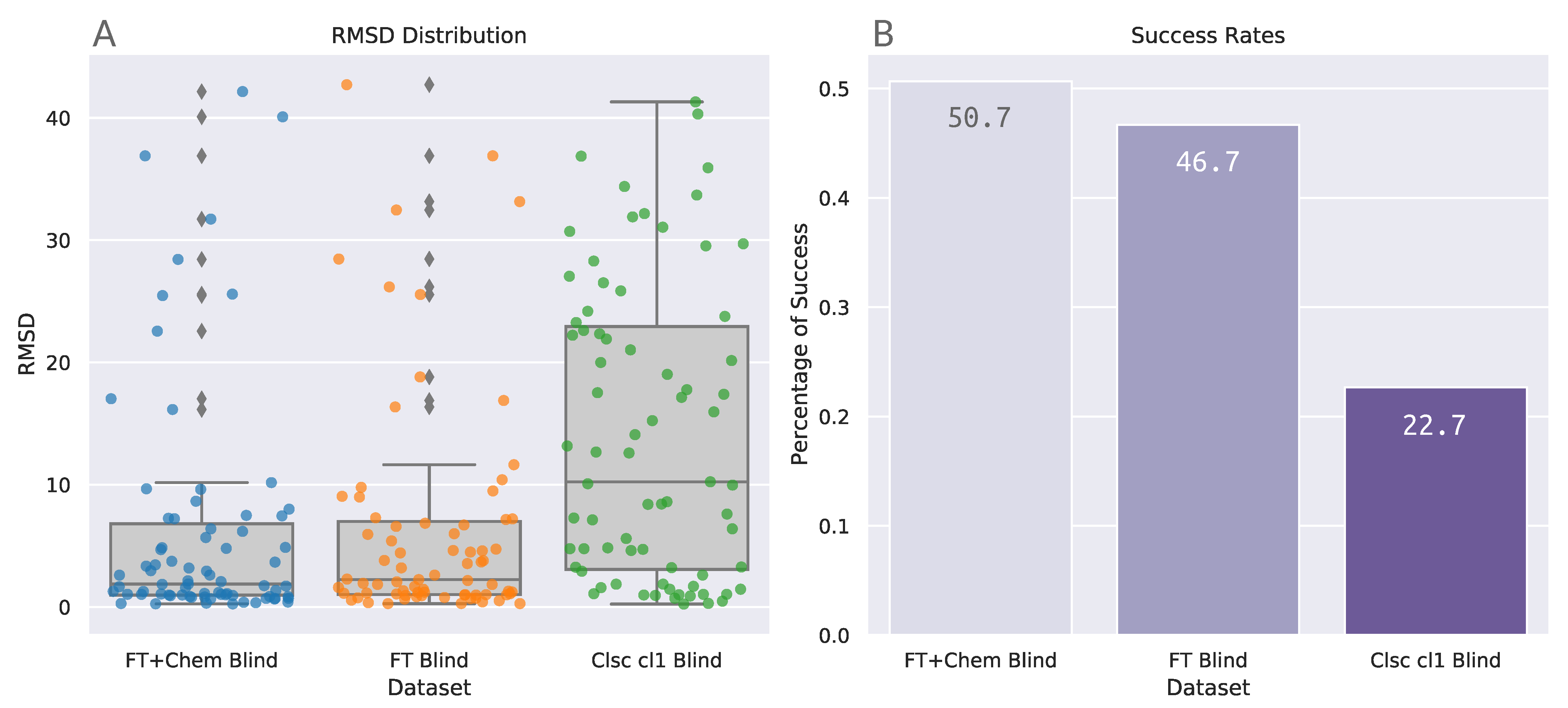
3.2. Astex Diverse Set
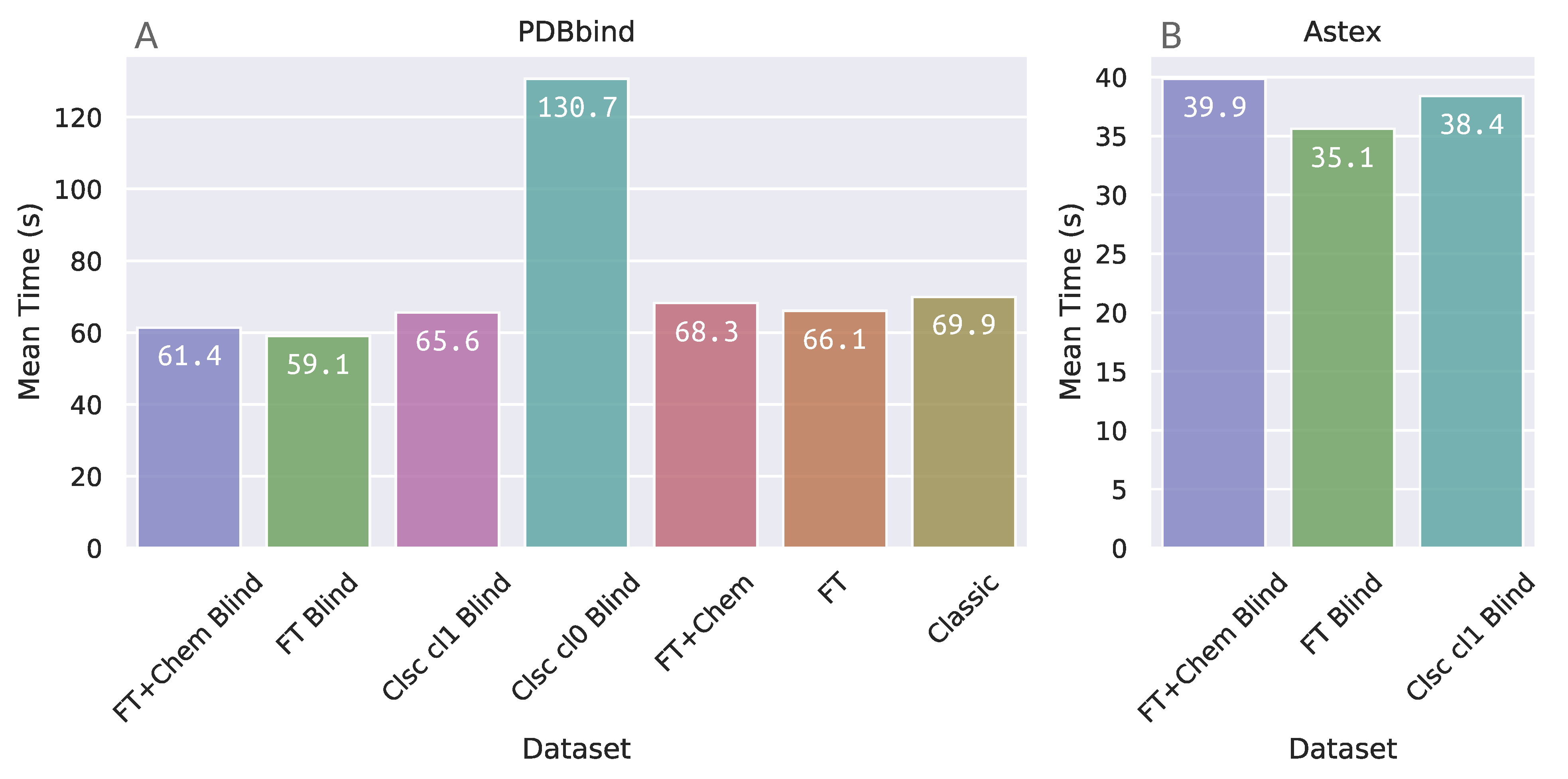
3.3. Docking Elapsed Time
4. Conclusions
Supplementary Materials
Author Contributions
Funding
Institutional Review Board Statement
Informed Consent Statement
Acknowledgments
Conflicts of Interest
References
- Torres, P.H.M.; Sodero, A.C.R.; Jofily, P.; Silva, F.P., Jr. Key Topics in Molecular Docking for Drug Design. Int. J. Mol. Sci. 2019, 20, 4574. [Google Scholar] [CrossRef] [PubMed]
- Ain, Q.U.; Aleksandrova, A.; Roessler, F.D.; Ballester, P.J. Machine-learning scoring functions to improve structure-based binding affinity prediction and virtual screening. Wiley Interdiscip. Rev. Comput. Mol. Sci. 2015, 5, 405–424. [Google Scholar] [CrossRef]
- Hassan, N.M.; Alhossary, A.A.; Mu, Y.; Kwoh, C.K. Protein-Ligand Blind Docking Using QuickVina-W with Inter-Process Spatio-Temporal Integration. Sci. Rep. 2017, 7, 15451. [Google Scholar] [CrossRef]
- Hetényi, C.; van der Spoel, D. Blind docking of drug-sized compounds to proteins with up to a thousand residues. FEBS Lett. 2006, 580, 1447–1450. [Google Scholar] [CrossRef] [PubMed]
- Hetényi, C.; van der Spoel, D. Efficient docking of peptides to proteins without prior knowledge of the binding site. Protein Sci. 2002, 11, 1729–1737. [Google Scholar] [CrossRef]
- Wu, Q.; Peng, Z.; Zhang, Y.; Yang, J. COACH-D: Improved protein-ligand binding sites prediction with refined ligand-binding poses through molecular docking. Nucleic Acids Res. 2018, 46, W438–W442. [Google Scholar] [CrossRef]
- Liu, Y.; Grimm, M.; Dai, W.T.; Hou, M.C.; Xiao, Z.X.; Cao, Y. CB-Dock: A web server for cavity detection-guided protein-ligand blind docking. Acta Pharmacol. Sin. 2020, 41, 138–144. [Google Scholar] [CrossRef]
- Morris, G.M.; Huey, R.; Lindstrom, W.; Sanner, M.F.; Belew, R.K.; Goodsell, D.S.; Olson, A.J. AutoDock4 and AutoDockTools4: Automated docking with selective receptor flexibility. J. Comput. Chem. 2009, 30, 2785–2791. [Google Scholar] [CrossRef]
- Trott, O.; Olson, A.J. AutoDock Vina: Improving the speed and accuracy of docking with a new scoring function, efficient optimization, and multithreading. J. Comput. Chem. 2009, 31, 455–461. [Google Scholar] [CrossRef]
- Jones, G.; Willett, P.; Glen, R.C.; Leach, A.R.; Taylor, R. Development and validation of a genetic algorithm for flexible docking. J. Mol. Biol. 1997, 267, 727–748. [Google Scholar] [CrossRef]
- Friesner, R.A.; Banks, J.L.; Murphy, R.B.; Halgren, T.A.; Klicic, J.J.; Mainz, D.T.; Repasky, M.P.; Knoll, E.H.; Shelley, M.; Perry, J.K.; et al. Glide: A New Approach for Rapid, Accurate Docking and Scoring. 1. Method and Assessment of Docking Accuracy. J. Med. Chem. 2004, 47, 1739–1749. [Google Scholar] [CrossRef]
- de Magalh aes, C.S.; Almeida, D.M.; Barbosa, H.J.C.; Dardenne, L.E. A dynamic niching genetic algorithm strategy for docking highly flexible ligands. Inf. Sci. 2014, 289, 206–224. [Google Scholar] [CrossRef]
- Ngan, C.H.; Hall, D.R.; Zerbe, B.; Grove, L.E.; Kozakov, D.; Vajda, S. FTSite: High accuracy detection of ligand binding sites on unbound protein structures. Bioinformatics 2012, 28, 286–287. [Google Scholar] [CrossRef] [PubMed]
- Xu, Y.; Wang, S.; Hu, Q.; Gao, S.; Ma, X.; Zhang, W.; Shen, Y.; Chen, F.; Lai, L.; Pei, J. CavityPlus: A web server for protein cavity detection with pharmacophore modelling, allosteric site identification and covalent ligand binding ability prediction. Nucleic Acids Res. 2018, 46, W374–W379. [Google Scholar] [CrossRef]
- Volkamer, A.; Kuhn, D.; Rippmann, F.; Rarey, M. DoGSiteScorer: A web server for automatic binding site prediction, analysis and druggability assessment. Bioinformatics 2012, 28, 2074–2075. [Google Scholar] [CrossRef]
- Jiménez, J.; Doerr, S.; Martínez-Rosell, G.; Rose, A.S.; De Fabritiis, G. DeepSite: Protein-binding site predictor using 3D-convolutional neural networks. Bioinformatics 2017, 33, 3036–3042. [Google Scholar] [CrossRef]
- Le Guilloux, V.; Schmidtke, P.; Tuffery, P. Fpocket: An open source platform for ligand pocket detection. BMC Bioinform. 2009, 10, 168. [Google Scholar] [CrossRef]
- Suplatov, D.; Kirilin, E.; Arbatsky, M.; Takhaveev, V.; Svedas, V. pocketZebra: A web-server for automated selection and classification of subfamily-specific binding sites by bioinformatic analysis of diverse protein families. Nucleic Acids Res. 2014, 42, W344–W349. [Google Scholar] [CrossRef]
- Grosdidier, A.; Zoete, V.; Michielin, O. SwissDock, a protein-small molecule docking web service based on EADock DSS. Nucleic Acids Res. 2011, 39, W270–W277. [Google Scholar] [CrossRef] [PubMed]
- Schneidman-Duhovny, D.; Inbar, Y.; Nussinov, R.; Wolfson, H.J. PatchDock and SymmDock: Servers for rigid and symmetric docking. Nucleic Acids Res. 2005, 33, W363–W367. [Google Scholar] [CrossRef]
- Lee, H.S.; Zhang, Y. BSP-SLIM: A blind low-resolution ligand-protein docking approach using predicted protein structures. Proteins 2012, 80, 93–110. [Google Scholar] [CrossRef] [PubMed]
- Ghersi, D.; Sanchez, R. Improving accuracy and efficiency of blind protein-ligand docking by focusing on predicted binding sites. Proteins 2009, 74, 417–424. [Google Scholar] [CrossRef] [PubMed]
- Grosdidier, A.; Zoete, V.; Michielin, O. Fast docking using the CHARMM force field with EADock DSS. J. Comput. Chem. 2011, 32, 2149–2159. [Google Scholar] [CrossRef] [PubMed]
- Kozakov, D.; Grove, L.E.; Hall, D.R.; Bohnuud, T.; Mottarella, S.E.; Luo, L.; Xia, B.; Beglov, D.; Vajda, S. The FTMap family of web servers for determining and characterizing ligand-binding hot spots of proteins. Nat. Protoc. 2015, 10, 733–755. [Google Scholar] [CrossRef] [PubMed]
- Pettersen, E.F.; Goddard, T.D.; Huang, C.C.; Couch, G.S.; Greenblatt, D.M.; Meng, E.C.; Ferrin, T.E. UCSF Chimera–a visualization system for exploratory research and analysis. J. Comput. Chem. 2004, 25, 1605–1612. [Google Scholar] [CrossRef] [PubMed]
- Allen, W.J.; Balius, T.E.; Mukherjee, S.; Brozell, S.R.; Moustakas, D.T.; Lang, P.T.; Case, D.A.; Kuntz, I.D.; Rizzo, R.C. DOCK 6: Impact of new features and current docking performance. J. Comput. Chem. 2015, 36, 1132–1156. [Google Scholar] [CrossRef]
- DOCK 6.9 User Manual. Available online: http://dock.compbio.ucsf.edu/DOCK_6/dock6_manual.htm#ChemicalMatching (accessed on 11 December 2020).
- JASP Team. JASP (Version 0.14) [Computer Software]. 2020. Available online: https://jasp-stats.org/ (accessed on 11 December 2020).


| FT+Chem | FT | Classic | Classic CL0 | Classic CL1 | |
|---|---|---|---|---|---|
| Site-specific | ✓ | ✓ | ✓ | ✗ | ✗ |
| Blind | ✓ | ✓ | ✗ | ✓ | ✓ |
| FT+Chem | FT | Classic | Classic CL0 | Classic CL1 | |
|---|---|---|---|---|---|
| Site-specific | ✓ | ✓ | ✓ | ✗ | ✗ |
| Blind | ✓ | ✓ | ✗ | ✓ | ✓ |
| FT+Chem Blind | FT Blind | Clsc cl1 Blind | Clsc cl0 Blind | FT+Chem | FT | Classic | |
|---|---|---|---|---|---|---|---|
| count | 157 | 157 | 157 | 157 | 157 | 157 | 157 |
| mean | 6.324 | 6.426 | 14.989 | 14.459 | 3.926 | 3.925 | 4.283 |
| std | 7.867 | 8.084 | 12.229 | 11.190 | 4.001 | 3.988 | 4.567 |
| min | 0.229 | 0.296 | 0.346 | 0.252 | 0.236 | 0.305 | 0.199 |
| 25% | 1.252 | 0.997 | 2.822 | 3.411 | 1.042 | 0.916 | 0.997 |
| 50% | 2.491 | 2.243 | 12.944 | 14.103 | 1.931 | 2.039 | 2.056 |
| 75% | 8.549 | 9.211 | 26.607 | 23.375 | 6.050 | 6.276 | 6.692 |
| max | 40.300 | 34.995 | 49.174 | 37.683 | 20.547 | 17.142 | 22.646 |
| Comparison | z | W | W | p | p | p |
|---|---|---|---|---|---|---|
| Clsc cl0 Blind-Clsc cl1 Blind | 0.069 | 381.140 | 379.736 | 0.473 | 1.000 | 0.848 |
| Clsc cl0 Blind-FT Blind | 6.570 | 381.140 | 246.599 | <0.001 | <0.001 | <0.001 |
| Clsc cl0 Blind-FT+Chem Blind | 6.378 | 381.140 | 250.525 | <0.001 | <0.001 | <0.001 |
| Clsc cl1 Blind-FT Blind | 6.502 | 379.736 | 246.599 | <0.001 | <0.001 | <0.001 |
| Clsc cl1 Blind-FT+Chem Blind | 6.310 | 379.736 | 250.525 | <0.001 | <0.001 | <0.001 |
| FT Blind-FT+Chem Blind | −0.192 | 246.599 | 250.525 | 0.424 | 1.000 | 0.848 |
| FT+Chem Blind | FT Blind | Clsc cl1 Blind | |
|---|---|---|---|
| count | 75 | 75 | 75 |
| mean | 6.241 | 6.438 | 14.085 |
| std | 9.720 | 9.375 | 11.999 |
| min | 0.246 | 0.272 | 0.236 |
| 25% | 0.958 | 1.005 | 3.065 |
| 50% | 1.877 | 2.238 | 10.235 |
| 75% | 6.804 | 6.996 | 22.936 |
| max | 42.148 | 42.713 | 41.307 |
| Comparison | z | W | W | p | p | p |
|---|---|---|---|---|---|---|
| Clsc cl1 Blind-FT Blind | 4.277 | 145.013 | 99.553 | <0.001 | <0.001 | <0.001 |
| Clsc cl1 Blind-FT+Chem Blind | 4.758 | 145.013 | 94.433 | <0.001 | <0.001 | <0.001 |
| FT Blind-FT+Chem Blind | 0.482 | 99.553 | 94.433 | 0.315 | 0.945 | 0.315 |
Publisher’s Note: MDPI stays neutral with regard to jurisdictional claims in published maps and institutional affiliations. |
© 2021 by the authors. Licensee MDPI, Basel, Switzerland. This article is an open access article distributed under the terms and conditions of the Creative Commons Attribution (CC BY) license (http://creativecommons.org/licenses/by/4.0/).
Share and Cite
Jofily, P.; Pascutti, P.G.; Torres, P.H.M. Improving Blind Docking in DOCK6 through an Automated Preliminary Fragment Probing Strategy. Molecules 2021, 26, 1224. https://doi.org/10.3390/molecules26051224
Jofily P, Pascutti PG, Torres PHM. Improving Blind Docking in DOCK6 through an Automated Preliminary Fragment Probing Strategy. Molecules. 2021; 26(5):1224. https://doi.org/10.3390/molecules26051224
Chicago/Turabian StyleJofily, Paula, Pedro G. Pascutti, and Pedro H. M. Torres. 2021. "Improving Blind Docking in DOCK6 through an Automated Preliminary Fragment Probing Strategy" Molecules 26, no. 5: 1224. https://doi.org/10.3390/molecules26051224
APA StyleJofily, P., Pascutti, P. G., & Torres, P. H. M. (2021). Improving Blind Docking in DOCK6 through an Automated Preliminary Fragment Probing Strategy. Molecules, 26(5), 1224. https://doi.org/10.3390/molecules26051224