
Anti-Cancer Drug Solubility Development within a Green Solvent: Design of Novel and Robust Mathematical Models Based on Artificial Intelligence


Abstract
:1. Introduction
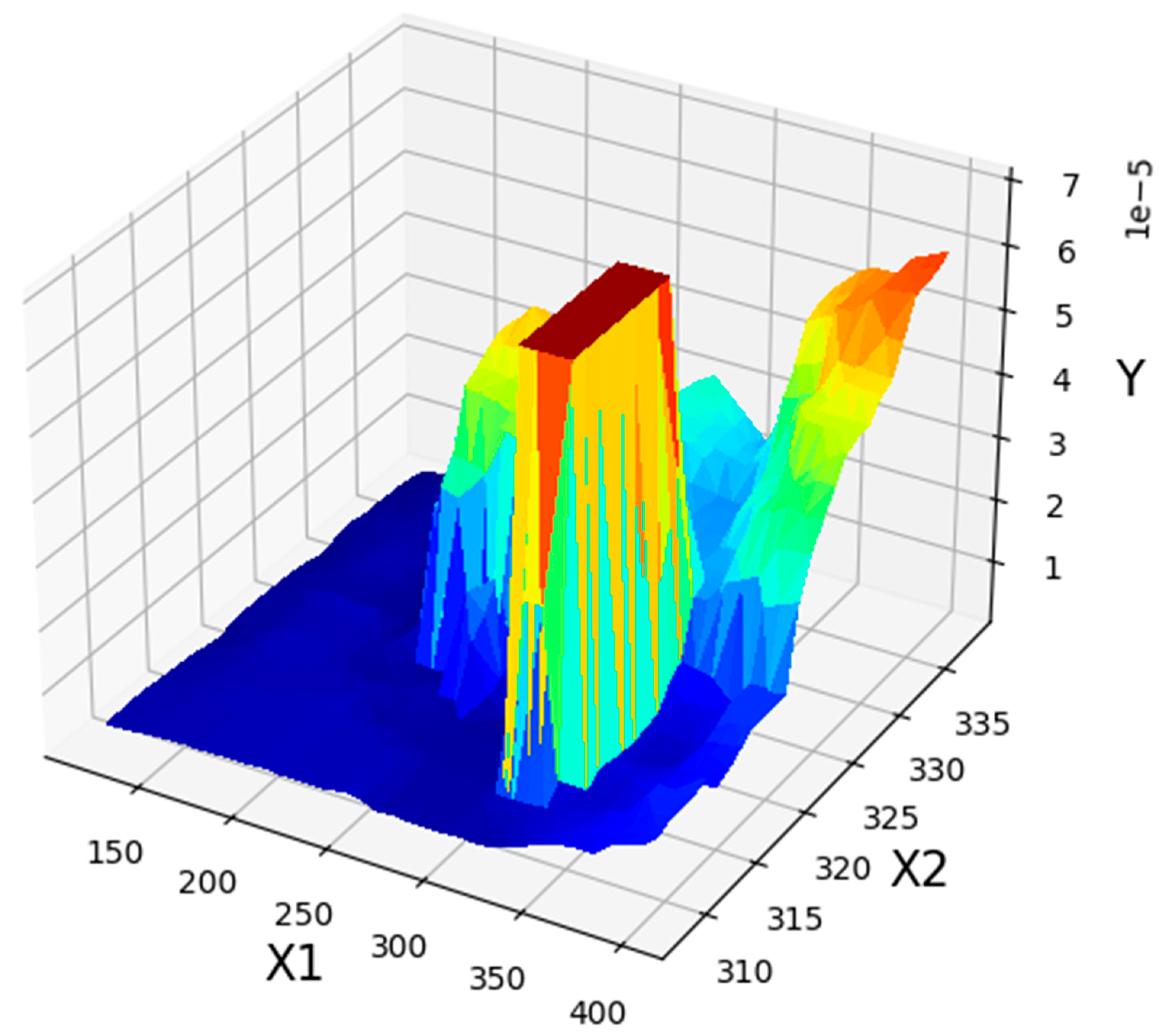
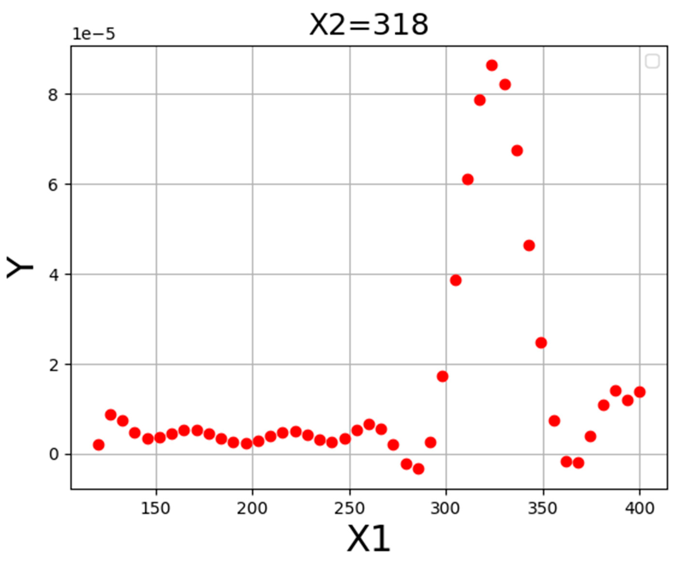
2. Dataset
3. Methodology
3.1. Base Models
- Inputs: training samples : input features, : real-valued output, testing point x to predict
- Algorithm:
- Calculate distance to every training example
- Select closet examples and their outputs
- Output:
3.2. AdaBoost
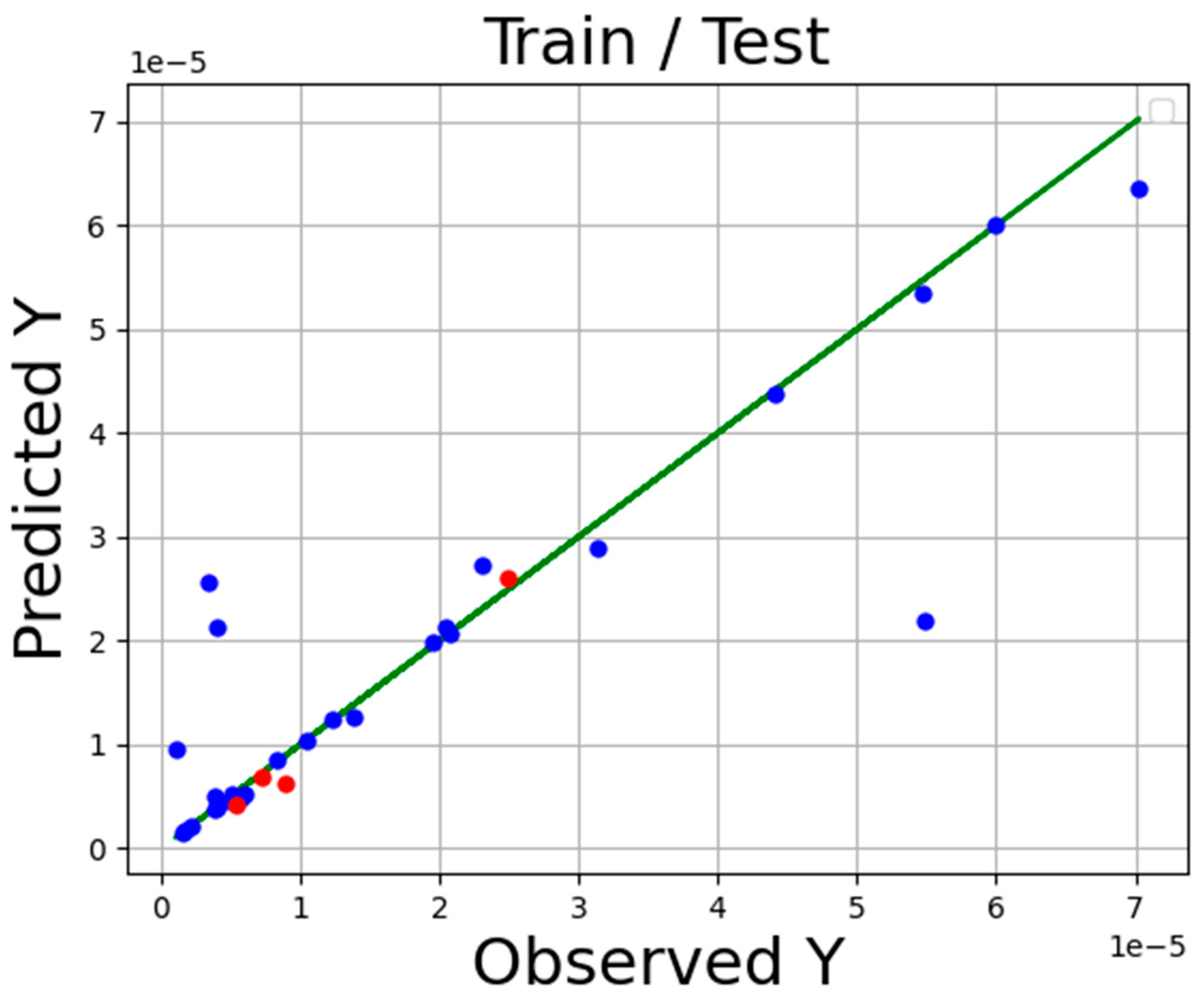
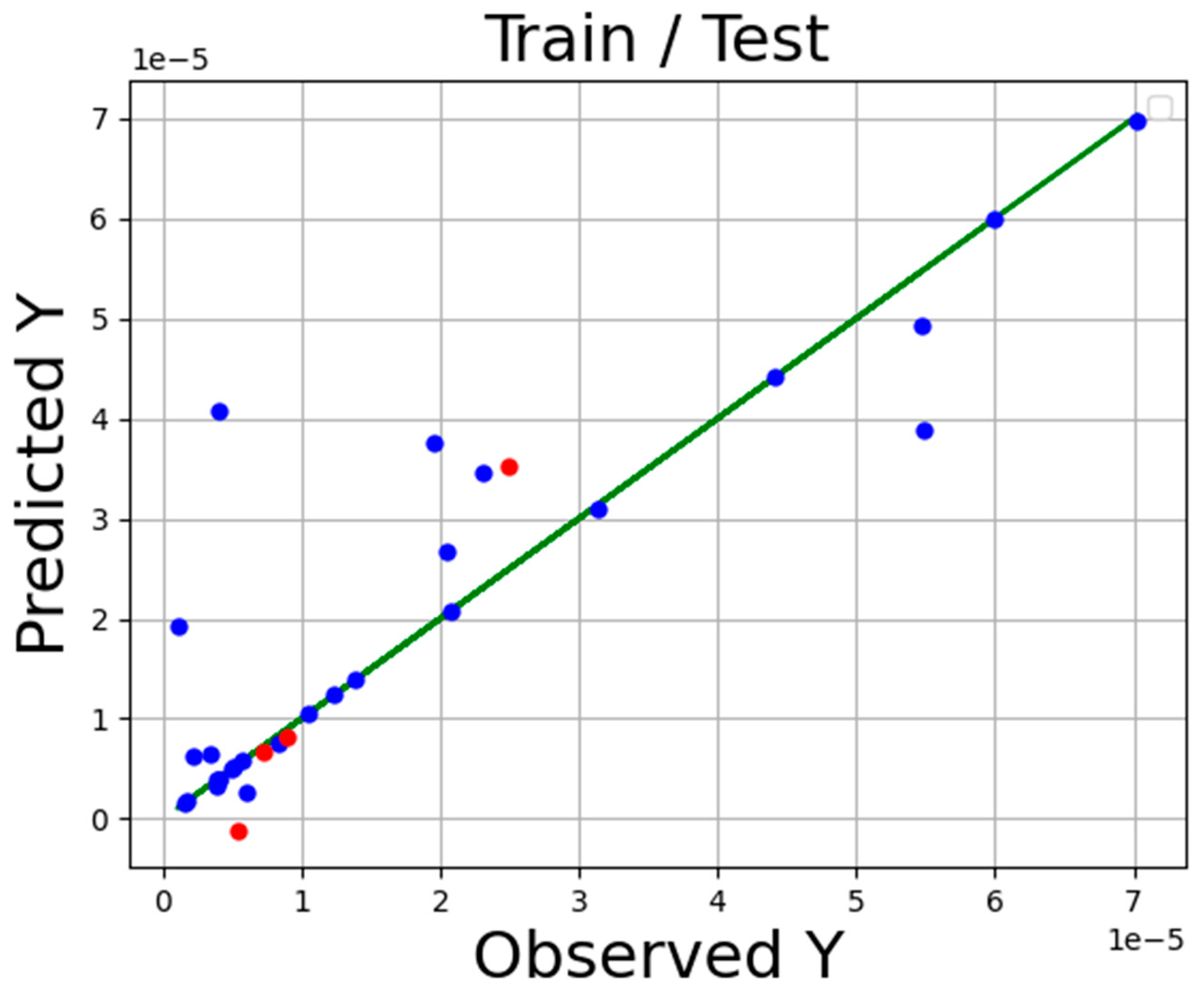
4. Results
5. Conclusions
Author Contributions
Funding
Institutional Review Board Statement
Informed Consent Statement
Data Availability Statement
Conflicts of Interest
References
- Faqi, A.S. A Comprehensive Guide to Toxicology in Nonclinical Drug Development; Academic Press: London, UK, 2016. [Google Scholar]
- Brun, R.; Don, R.; Jacobs, R.T.; Wang, M.Z.; Barrett, M.P. Development of novel drugs for human African trypanosomiasis. Future Microbiol. 2011, 6, 677–691. [Google Scholar] [CrossRef]
- Martell, R.E.; Brooks, D.G.; Wang, Y.; Wilcoxen, K. Discovery of novel drugs for promising targets. Clin. Ther. 2013, 35, 1271–1281. [Google Scholar] [CrossRef]
- Mirhaji, E.; Afshar, M.; Rezvani, S.; Yoosefian, M. Boron nitride nanotubes as a nanotransporter for anti-cancer docetaxel drug in water/ethanol solution. J. Mol. Liq. 2018, 271, 151–156. [Google Scholar] [CrossRef]
- Savjani, K.T.; Gajjar, A.K.; Savjani, J.K. Drug solubility: Importance and enhancement techniques. Int. Sch. Res. Not. 2012, 2012, 195727. [Google Scholar] [CrossRef] [PubMed]
- Gorain, B.; Pandey, M.; Choudhury, H.; Jain, G.K.; Kesharwani, P. Dendrimer for solubility enhancement. In Dendrimer-Based Nanotherapeutics; Elsevier: Amsterdam, The Netherlands, 2021; pp. 273–283. [Google Scholar]
- Williams, H.D.; Trevaskis, N.L.; Charman, S.A.; Shanker, R.M.; Charman, W.N.; Pouton, C.W.; Porter, C.J.H. Strategies to address low drug solubility in discovery and development. Pharmacol. Rev. 2013, 65, 315–499. [Google Scholar] [CrossRef]
- Vimalson, D.C. Techniques to enhance solubility of hydrophobic drugs: An overview. Asian J. Pharm. 2016, 10. [Google Scholar] [CrossRef]
- Das, B.; Baidya, A.T.; Mathew, A.T.; Yadav, A.K.; Kumar, R. Structural modification aimed for improving solubility of lead compounds in early phase drug discovery. Bioorganic Med. Chem. 2022, 56, 116614. [Google Scholar] [CrossRef] [PubMed]
- Bagade, O.; Kad, D.R.; Bhargude, D.N.; Bhosale, D.R.; Kahane, S.K. Consequences and impose of solubility enhancement of poorly water soluble drugs. Res. J. Pharm. Technol. 2014, 7, 598. [Google Scholar]
- Cao, M.; Yoosefian, D.W.M.; Sabaei, S.; Jahani, M. Comprehensive study of the encapsulation of Lomustine anticancer drug into single walled carbon nanotubes (SWCNTs): Solvent effects, molecular conformations, electronic properties and intramolecular hydrogen bond strength. J. Mol. Liq. 2020, 320, 114285. [Google Scholar] [CrossRef]
- Girotra, P.; Singh, S.K.; Nagpal, K. Supercritical fluid technology: A promising approach in pharmaceutical research. Pharm. Dev. Technol. 2013, 18, 22–38. [Google Scholar] [CrossRef]
- Macnaughton, S.J.; Kikic, I.; Foster, N.R.; Alessi, P.; Cortesi, A.; Colombo, I. Solubility of anti-inflammatory drugs in supercritical carbon dioxide. J. Chem. Eng. Data 1996, 41, 1083–1086. [Google Scholar] [CrossRef]
- Zhou, M.; Ni, R.; Zhao, Y.; Huang, J.; Deng, X. Research progress on supercritical CO2 thickeners. Soft Matter 2021, 1, 5107–5115. [Google Scholar] [CrossRef] [PubMed]
- Baldino, L.; Cardea, S.; Reverchon, E. Biodegradable membranes loaded with curcumin to be used as engineered independent devices in active packaging. J. Taiwan Inst. Chem. Eng. 2017, 71, 518–526. [Google Scholar] [CrossRef]
- Su, W.; Zhang, H.; Xing, Y.; Li, X.; Wang, J.; Cai, C. A bibliometric analysis and review of supercritical fluids for the synthesis of nanomaterials. Nanomaterials 2021, 11, 336. [Google Scholar] [CrossRef]
- Baldino, L.; della Porta, G.; Reverchon, E. Supercritical CO2 processing strategies for pyrethrins selective extraction. J. CO2 Util. 2017, 20, 14–19. [Google Scholar] [CrossRef]
- Yoosefian, M.; Sabaei, S.; Etminan, N. Encapsulation efficiency of single-walled carbon nanotube for Ifosfamide anti-cancer drug. Comput. Biol. Med. 2019, 114, 103433. [Google Scholar] [CrossRef] [PubMed]
- Zhu, H.; Zhu, L.; Sun, Z.; Khan, A. Machine learning based simulation of an anti-cancer drug (busulfan) solubility in supercritical carbon dioxide: ANFIS model and experimental validation. J. Mol. Liq. 2021, 338, 116731. [Google Scholar] [CrossRef]
- Öztürk, A.A.; Gündüz, A.B.; Ozisik, O. Supervised machine learning algorithms for evaluation of solid lipid nanoparticles and particle size. Comb. Chem. High Throughput Screen. 2018, 21, 693–699. [Google Scholar] [CrossRef] [PubMed]
- Staszak, M. Artificial intelligence in the modeling of chemical reactions kinetics. Phys. Sci. Rev. 2020. [Google Scholar] [CrossRef]
- Wang, X.; Luo, L.; Xiang, J.; Zheng, S.; Shittu, S.; Wang, Z.; Zhao, X. A comprehensive review on the application of nanofluid in heat pipe based on the machine learning: Theory, application and prediction. Renew. Sustain. Energy Rev. 2021, 150, 111434. [Google Scholar] [CrossRef]
- Lazzús, J.A.; Cuturrufo, F.; Pulgar-Villarroel, G.; Salfate, I.; Vega, P. Estimating the temperature-dependent surface tension of ionic liquids using a neural network-based group contribution method. Ind. Eng. Chem. Res. 2017, 56, 6869–6886. [Google Scholar] [CrossRef]
- Murphy, K.P. Machine Learning: A Probabilistic Perspective; MIT Press: Cambridge, MA, USA, 2012. [Google Scholar]
- Mitchell, T.M. The Discipline of Machine Learning; Carnegie Mellon University: Pittsburgh, PA, USA, 2006; Volume 9. [Google Scholar]
- El Naqa, I.; Murphy, M.J. What is machine learning? In Machine Learning in Radiation Oncology; Springer: Berlin/Heidelberg, Germany, 2015; pp. 3–11. [Google Scholar]
- Goodfellow, I.; Bengio, Y.; Courville, A. Machine learning basics. Deep. Learn. 2016, 1, 98–164. [Google Scholar]
- Shehadeh, A.; Alshboul, O.; Al Mamlook, R.E.; Hamedat, O. Machine learning models for predicting the residual value of heavy construction equipment: An evaluation of modified decision tree, LightGBM, and XGBoost regression. Autom. Constr. 2021, 129, 103827. [Google Scholar] [CrossRef]
- Freund, Y.; Schapire, R.E. A decision-theoretic generalization of on-line learning and an application to boosting. J. Comput. Syst. Sci. 1997, 55, 119–139. [Google Scholar] [CrossRef]
- Rasmussen, C.E. Gaussian processes in machine learning. In Summer School on Machine Learning; Springer: Berlin/Heidelberg, Germany, 2003. [Google Scholar]
- Shi, J.Q.; Choi, T. Gaussian Process Regression Analysis for Functional Data; CRC Press: Boca Raton, FL, USA, 2011. [Google Scholar]
- Masegosa, R.A.; Armañanzas, R.; Abad-Grau, M.M.; Potenciano, V.; Moral, S.; Larrañaga, P.; Bielza, C.; Matesanz, F. Discretization of Expression Quantitative Trait Loci in Association Analysis Between Genotypes and Expression Data. Curr. Bioinform. 2015, 10, 144–164. [Google Scholar] [CrossRef]
- Wilcox, R. A note on the Theil-Sen regression estimator when the regressor is random and the error term is heteroscedastic. Biom. J. 1998, 40, 261–268. [Google Scholar] [CrossRef]
- Ohlson, J.A.; Kim, S. Linear valuation without OLS: The Theil-Sen estimation approach. Rev. Account. Stud. 2015, 20, 395–435. [Google Scholar] [CrossRef]
- Pishnamazi, M.; Zabihi, S.; Jamshidian, S.; Borousan, F.; Hezave, A.Z.; Shirazian, S. Thermodynamic modelling and experimental validation of pharmaceutical solubility in supercritical solvent. J. Mol. Liq. 2020, 319, 114120. [Google Scholar] [CrossRef]
- Williams, C.K.; Rasmussen, C.E. Gaussian Processes for Regression; 1996. [Google Scholar]
- Rasmussen, C.E. Evaluation of Gaussian Processes and Other Methods for Non-Linear Regression; University of Toronto: Toronto, ON, Canada, 1997. [Google Scholar]
- Taherdangkoo, R.; Yang, H.; Akbariforouz, M.; Sun, Y.; Liu, Q.; Butscher, C. Gaussian process regression to determine water content of methane: Application to methane transport modeling. J. Contam. Hydrol. 2021, 243, 103910. [Google Scholar] [CrossRef]
- Alghamdi, A.S.; Polat, K.; Alghoson, A.; Alshdadi, A.A.; Abd El-Latif, A.A. Gaussian process regression (GPR) based non-invasive continuous blood pressure prediction method from cuff oscillometric signals. Appl. Acoust. 2020, 164, 107256. [Google Scholar] [CrossRef]
- Cheng, M.; Prayogo, D. Optimizing Biodiesel Production from Rice Bran Using Artificial Intelligence Approaches; Department of Construction Engineering, National Taiwan University of Science and Technology: Taipei, Taiwan, 2016. [Google Scholar]
- Williams, C.K.; Barber, D. Bayesian classification with Gaussian processes. IEEE Trans. Pattern Anal. Mach. Intell. 1998, 20, 1342–1351. [Google Scholar] [CrossRef]
- Cover, T. Estimation by the nearest neighbor rule. IEEE Trans. Inf. Theory 1968, 14, 50–55. [Google Scholar] [CrossRef]
- Song, Y.; Liang, J.; Lu, J.; Zhao, X. An efficient instance selection algorithm for k nearest neighbor regression. Neurocomputing 2017, 251, 26–34. [Google Scholar] [CrossRef]
- Sen, P.K. Estimates of the regression coefficient based on Kendall’s tau. J. Am. Stat. Assoc. 1968, 63, 1379–1389. [Google Scholar] [CrossRef]
- Caloiero, T.; Aristodemo, F.; Ferraro, D.A. Annual and seasonal trend detection of significant wave height, energy period and wave power in the Mediterranean Sea. Ocean. Eng. 2022, 243, 110322. [Google Scholar] [CrossRef]
- Freund, Y.; Schapire, R.E. Experiments with a new boosting algorithm. In Proceedings of the Thirteenth International Conference on International Conference on Machine Learning, Bari, Italy, 3–6 July 1996; Citeseer: Princeton, NJ, USA, 1996. [Google Scholar]
- Drucker, H. Improving regressors using boosting techniques. In Proceedings of the Fourteenth International Conference on Machine Learning, San Francisco, CA, USA, 8–12 July 1997; Citeseer: Princeton, NJ, USA, 1997. [Google Scholar]
- Dargahi-Zarandi, A.; Hemmati-Sarapardeh, A.; Shateri, M.; Menad, N.A.; Ahmadi, M. Modeling minimum miscibility pressure of pure/impure CO2-crude oil systems using adaptive boosting support vector regression: Application to gas injection processes. J. Pet. Sci. Eng. 2020, 184, 106499. [Google Scholar] [CrossRef]
- Wu, Q.; Burges, C.J.C.; Svore, K.M.; Gao, J. Adapting boosting for information retrieval measures. Inf. Retr. 2010, 13, 254–270. [Google Scholar] [CrossRef]
- Ying, C.; Miao, Q.; Liu, J.; Gao, L. Advance and prospects of AdaBoost algorithm. Acta Autom. Sin. 2013, 39, 745–758. [Google Scholar]
- Botchkarev, A. Evaluating Performance of Regression Machine Learning Models Using Multiple Error Metrics in Azure Machine Learning Studio. 2018. Available online: https://papers.ssrn.com/sol3/papers.cfm?abstract_id=3177507 (accessed on 9 August 2022).
- Kumar, S.; Mishra, S.; Singh, S.K. A machine learning-based model to estimate PM2. 5 concentration levels in Delhi’s atmosphere. Heliyon 2020, 6, e05618. [Google Scholar] [CrossRef]


| No. | X1 = P (bar) | X2 = T (K) | Y (Solubility/Mole Fraction) |
|---|---|---|---|
| 1 | 120 | 308 | 4 × 10⁻⁶ |
| 2 | 160 | 308 | 4.94 × 10⁻⁶ |
| 3 | 200 | 308 | 5.49 × 10⁻⁶ |
| 4 | 240 | 308 | 5.96 × 10⁻⁶ |
| 5 | 280 | 308 | 3.99 × 10⁻⁶ |
| 6 | 320 | 308 | 3.88 × 10⁻⁶ |
| 7 | 360 | 308 | 8.38 × 10⁻⁶ |
| 8 | 400 | 308 | 1.24 × 10⁻⁵ |
| 9 | 120 | 318 | 2.15 × 10⁻⁶ |
| 10 | 160 | 318 | 5.79 × 10⁻⁶ |
| 11 | 200 | 318 | 8.95 × 10⁻⁶ |
| 12 | 240 | 318 | 7.27 × 10⁻⁶ |
| 13 | 280 | 318 | 3.40 × 10⁻⁶ |
| 14 | 320 | 318 | 7.03 × 10⁻⁵ |
| 15 | 360 | 318 | 4.01 × 10⁻⁶ |
| 16 | 400 | 318 | 1.39 × 10⁻⁵ |
| 17 | 120 | 328 | 1.79 × 10⁻⁶ |
| 18 | 160 | 328 | 5.13 × 10⁻⁶ |
| 19 | 200 | 328 | 1.05 × 10⁻⁶ |
| 20 | 240 | 328 | 5.48 × 10⁻⁵ |
| 21 | 280 | 328 | 2.31 × 10⁻⁵ |
| 22 | 320 | 328 | 2.04 × 10⁻⁵ |
| 23 | 360 | 328 | 2.50 × 10⁻⁵ |
| 24 | 400 | 328 | 4.41 × 10⁻⁵ |
| 25 | 120 | 338 | 1.52 × 10⁻⁵ |
| 26 | 160 | 338 | 3.84 × 10⁻⁶ |
| 27 | 200 | 338 | 1.05 × 10⁻⁵ |
| 28 | 240 | 338 | 2.08 × 10⁻⁵ |
| 29 | 280 | 338 | 3.13 × 10⁻⁵ |
| 30 | 320 | 338 | 1.95 × 10⁻⁵ |
| 31 | 360 | 338 | 5.47 × 10⁻⁵ |
| 32 | 400 | 338 | 6.0 × 10⁻⁵ |
| Models | MAE | R2 |
|---|---|---|
| ADA-KNN | 1.98 × 10⁻⁶ | 0.996 |
| ADA-GPR | 1.33 × 10⁻⁶ | 0.967 |
| ADA-TSR | 2.33 × 10⁻⁶ | 0.883 |
| X1 = P (bar) | X2 = T (K) | Y (Solubility) |
|---|---|---|
| 329 | 318.0 | 7.03 × 10⁻⁵ |
Publisher’s Note: MDPI stays neutral with regard to jurisdictional claims in published maps and institutional affiliations. |
© 2022 by the authors. Licensee MDPI, Basel, Switzerland. This article is an open access article distributed under the terms and conditions of the Creative Commons Attribution (CC BY) license (https://creativecommons.org/licenses/by/4.0/).
Share and Cite
Huwaimel, B.; Alobaida, A. Anti-Cancer Drug Solubility Development within a Green Solvent: Design of Novel and Robust Mathematical Models Based on Artificial Intelligence. Molecules 2022, 27, 5140. https://doi.org/10.3390/molecules27165140
Huwaimel B, Alobaida A. Anti-Cancer Drug Solubility Development within a Green Solvent: Design of Novel and Robust Mathematical Models Based on Artificial Intelligence. Molecules. 2022; 27(16):5140. https://doi.org/10.3390/molecules27165140
Chicago/Turabian StyleHuwaimel, Bader, and Ahmed Alobaida. 2022. "Anti-Cancer Drug Solubility Development within a Green Solvent: Design of Novel and Robust Mathematical Models Based on Artificial Intelligence" Molecules 27, no. 16: 5140. https://doi.org/10.3390/molecules27165140