Article

Naive Prediction of Protein Backbone Phi and Psi Dihedral Angles Using Deep Learning

1
Faculty of Chemistry and Chemical Engineering, University of Maribor, Smetanova ulica 17, SI-2000 Maribor, Slovenia
2
Faculty of Mathematics, Natural Sciences and Information Technologies, University of Primorska, Glagoljaška ulica 8, SI-6000 Koper, Slovenia
3
Institute of Environmental Protection and Sensors, Beloruska ulica 7, SI-2000 Maribor, Slovenia
*
Authors to whom correspondence should be addressed.
Molecules 2023, 28(20), 7046; https://doi.org/10.3390/molecules28207046
Submission received: 1 September 2023 / Revised: 6 October 2023 / Accepted: 9 October 2023 / Published: 12 October 2023

Abstract

:
Protein structure prediction represents a significant challenge in the field of bioinformatics, with the prediction of protein structures using backbone dihedral angles recently achieving significant progress due to the rise of deep neural network research. However, there is a trend in protein structure prediction research to employ increasingly complex neural networks and contributions from multiple models. This study, on the other hand, explores how a single model transparently behaves using sequence data only and what can be expected from the predicted angles. To this end, the current paper presents data acquisition, deep learning model definition, and training toward the final protein backbone angle prediction. The method applies a simple fully connected neural network (FCNN) model that takes only the primary structure of the protein with a sliding window of size 21 as input to predict protein backbone ϕ and ψ dihedral angles. Despite its simplicity, the model shows surprising accuracy for the ϕ angle prediction and somewhat lower accuracy for the ψ angle prediction. Moreover, this study demonstrates that protein secondary structure prediction is also possible with simple neural networks that take in only the protein amino-acid residue sequence, but more complex models are required for higher accuracies.

Graphical Abstract

1. Introduction

Proteins are commonly composed of 20 natural amino acid residues, which together form the primary protein structure. Each amino-acid residue contains the common atoms N, Cα, and C that comprise the protein backbone, or main chain. As illustrated in Figure 1, the backbone structure of amino-acid residues can be described by sets of ϕ (phi), ψ (psi), and ω (omega) dihedral angles. These angles are defined by considering four consecutive backbone atoms from the sequence Ci−1, Ni, Cαi, Ci, Ni+1, and Cαi+1. In order to simplify models, the ω angle can be typically fixed at 180° [1]. Each amino-acid residue has a side chain emanating from its Cα atom; however, secondary structure prediction studies typically disregard it and rather focus on the protein backbone.
Predicting the three-dimensional structure of a given protein from its sequence, known as protein structure prediction (PSP), has presented a major challenge in biochemistry for decades. In 2020, DeepMind released AlphaFold, which has become the most accurate algorithm to date for tackling this problem [2]. AlphaFold’s exceptional performance in the free modeling (FM) section of the thirteenth critical assessment of protein structure prediction (CASP) ignited heightened public interest [3,4]. At CASP14, the most up-to-date variant of AlphaFold entered under the group name “AlphaFold2”, showed tremendous progress in accuracy, thereby setting a new benchmark for sub-Ångström root mean square deviation (Cα r.m.s.d.) backbone predictions [5,6]. Before AlphaFold revolutionized PSP, numerous algorithms for accurately predicting protein secondary structure were developed and remain indispensable, both for template-free and template-based protein structure predictions [6,7,8,9,10].
Protein secondary structure prediction (PSSP) is commonly viewed as a categorization problem wherein each amino acid residue is classified according to its secondary structure type. PSSP models accept a sequence of amino-acid residues as input and return the corresponding sequence of secondary structures. They can be classified into several types depending on the number of secondary structure categories, with three-state (Q3) and eight-state (Q8) models being the most common. In the three-state PSSP model, the secondary structure elements are composed of two main conformations, helix (H) and sheet (E) [11], plus the coil (C) category representing the amino-acid residues that fall into neither of the previous two categories. The eight-state PSSP framework, on the other hand, incorporates eight categories of protein secondary structures: α-helix (H), 310-helix (G), parallel/anti-parallel β-sheet conformation (E), isolated β-bridge (B), bend (S), turn (T), π-helix (I), and coil (C) categories, as initially proposed by Kabsch and Sander [12]. Another approach for the classification of protein structures is DISICL [13], a dihedral-based segment identification and classification method that offers 18 distinct structural classes, which can be simplified into seven more general classes, providing a detailed analysis of subtle structural changes. Over the years, numerous methods and algorithms have been developed that reached 70.2–87.3% Q3 accuracies (PHD [14], PSIPRED [15], SPINE [16,17], SPARROW [18], Porter 4.0 [19], SCORPION [20], SPIDER2 [21], Jpred4 [22,23], DeepCNF [24], SPIDER3 [25], MUFOLD-SS [26], NetSurfP-2.0 [27], CRRNN and eCRRNN [28], OPUS-TASS [29], and DNSS2 [30]), but lower Q8 accuracies ranging from 62.6% to 76.5% (SSpro8 [31], RaptorX-SS8 [32], SCORPION [33], ICML2014 [34], DeepCNF [24], MUFOLD-SS [26], CRRNN and eCRRNN [28]), owing to the increasing complexity of the problem.
Despite the recent improvements in predicting ϕ and ψ backbone angles, the obtained ranges of indicative angles are still relatively wide (approximately 20°), which poses a significant challenge when attempting to capture the protein backbone structure accurately. Various methods have been proposed to predict backbone angles as continuous or discrete labels, with the aim of achieving increased accuracy compared to secondary structure prediction for application in ab initio structure prediction or refinement [35,36]. Recent advances in protein backbone angle predictions (BAP) have been made through the use of deep neural networks (DNNs). DNN variants, such as stacked sparse auto-encoder neural networks [37], long short-term memory (LSTM), bidirectional recurrent neural networks (BRNNs) [25,29,38], residual networks (ResNets) [38], and DNN ensembles [29,38] or layered iterations [21], have been utilized for BAP. Common input features for BAP include position-specific scoring matrices (PSSMs) [21,37,38,39,40,41] generated by PSI-BLAST, 7 physicochemical properties (7PCP) [21,37,38,40], such as hydrophobicity and volume, predicted accessible surface area (ASA) [37,41], hidden Markov model (HMM) profiles [27,38,40] (by HHBlits [42]), contact maps [38], and PSP19 [29]. Additionally, to capture local structures around amino-acid residues, many methods use sliding windows [21,25,37,41], while others apply entire protein sequences as features [21,43] to capture long-range interactions. Convolutional neural networks (CNNs) [27,29] or LSTM-BRNNs [25,38] have also been utilized for this purpose.
However, despite these advancements, more accurate BAP is still needed due to the cascading effect of errors at any angle of a protein structure. Consequently, other methods for BAP have been developed, such as ANGLOR [41], SPIDER [37], SPIDER2 [21], SPIDER3 [25], SPOT—Contact [44], RaptorX-Angle [45], DeepRIN [19], NetSurfP-2.0 [27], SPOT-1D [38], OPUS-TASS [29], and SAP [46]. For example, ANGLOR utilizes neural networks and support vector machines (SVMs) [31] to predict ϕ and ψ angles separately, while SPIDER applies a stacked sparse autoencoder DNN for predicting θ (planar angle defined by the consecutive Cα atoms) and τ (dihedral angle defined by four consecutive Cα atoms) angles. RaptorX-Angle uses a combination of clustering and deep learning to predict ϕ and ψ values, and DeepRIN utilizes a deep residual inception network for the same purpose. NetSurfP-2.0, on the other hand, employs large LSTM networks in BRNNs to predict ϕ and ψ angles. Moreover, SPOT-1D applies an ensemble of LSTM-BRNN and ResNets with input features PSSM, HMM, 7PCP, and contact maps; the contact maps are taken from SPOT-Contact [44] and are used in a sliding window fashion. Entire proteins are also applied as features for SPOT-1D. OPUS-TASS predicts only ϕ and ψ angles with ensembles of DNNs having CNN, LSTM, and Transformer [32] layers. It utilizes an input feature called PSP19 [33] that classifies residues into rigid-body blocks and a constrained feature called CSF3 [34] to describe backbone structures. OPUS-TASS also employs a multi-task learning strategy [35]. SAP predicts all four types of backbone angles using a simple fully connected neural network (FCNN) with sliding windows, 8-state SS predictions, PSSM, and 7PCP input features. On the benchmark datasets, SAP4SS [47] has achieved mean absolute error (MAE) values of 15.59°, 18.87°, 6.03°, and 21.71°, respectively, for ϕ, ψ, θ, and τ predictions, which is a slight improvement from SAP [46], which has achieved values of 15.65°, 18.59°, 6.07°, and 21.03°, respectively. As a result, SAP4SS has somewhat outperformed the existing state-of-the-art methods such as SAP, SPOT-1D, and OPUS-TASS, with differences in MAE ranging from 1.5 to 4.1% compared to the best-known results.
The current study applies a simple fully connected neural network (FCNN) that takes only a given primary structure of the protein with a sliding window of size 21 as input features to predict ϕ and ψ angles. Despite its simplicity, the model predicts ϕ dihedral angles with a surprising accuracy of 23.53° MAE but performs somewhat worse for the prediction of ψ dihedral angles (MAE of 44.14°). The study shows that even a naive approach to a simple model can perform with surprising accuracy and can serve to study the primary sequence of proteins while maintaining the transparency of the model and a good overview of the input data. This study also serves to demonstrate how a simple model based on sequence input data could integrate into complex ensemble solutions like AlphaFold.

2. Results

Upon finishing model training, the ϕ and ψ angle predictions were made for the test dataset. For each prediction, the loss function formula was applied so that the error calculation accounted for the angle periodicity, and all predicted angles were adjusted either by adding or subtracting 360° so that they fell into the same −180° to 180° range as the measured angles. The results were analyzed using custom Python functions using the Pandas 1.5.1. package [48] for the dataset handling and MatPlotLib 3.6.3 [49] for the graphs.

2.1. Mean Absolute Prediction Error

Figure 2 shows that the distribution of the neural network model predicted values corresponds to the distribution of the measured values for ψ and ϕ angles, with peaks and troughs in both distributions aligning across the range. However, the predicted distributions’ peaks are larger and narrower than the measured distribution peaks, while the predicted distributions’ troughs are wider than the ones of the measured distributions, effectively resulting in a smoothed lower-resolution distribution curve. The neural network model therefore produces similar angle distributions as the ones obtained by the SAP4SS beforehand [47] (depicted in Figure 2).
In Figure 2, where angle distributions are depicted, the peaks represent well-defined secondary structures, such as helices and sheets. The ϕ distribution is heavily skewed toward negative dihedral angle values because the three common secondary structure elements overlap there—right-handed α-helix, 310-helix, and β-sheet—while the small peak around 40° to 100° corresponds to the left-handed α-helix. Conversely, the ψ angle distributions are more evenly divided into two peaks, corresponding to the two most prominent secondary structure elements—right-handed α-helix and β-sheet. Herein, the reason behind less accurate predictions of ψ angles by neural networks can be clearly visualized.
For each data row, the mean absolute error (MAE) was determined by utilizing the already-described loss function formula. The mean absolute error and its corresponding standard deviation were then calculated for all 20 amino-acid residues (Figure 3). The resulting mean absolute error was 23.53° for ϕ angles and 44.14° for ψ angles. An important trend can be observed from Figure 3, namely that predictions of phi angles exhibit greater accuracy when compared to psi angles (with the notable exception of glycine).
The poor performance of ψ predictions compared to ϕ predictions originates from the differences in the input data. Namely, as observed beforehand, ϕ and ψ exhibit different distribution patterns, with ϕ presenting a peak at around −90° and an effective distribution of approximately 100°, while ψ possesses two peaks at −110° and 130° with an approximate distribution of 150° (Figure 2). Figure S1 also illustrates that the standard deviation of proline ϕ angles is the smallest (10.93°) in the dataset, as expected, due to the cyclic proline structure, while the standard deviation of glycine ϕ angles is the largest (96.21°), with the average for all remaining amino-acid residues of 39.60° (Table S1). This difference in the measured angle deviations between amino-acid residues corresponds to the pattern observed in the mean absolute prediction error of ϕ angles per amino-acid residue—the proline ϕ angles were the easiest to predict with the mean prediction error of 7.77°, while the small and flexible glycine was the most difficult to predict with the mean prediction error of 58.72°. The differences in the MAE of predictions for ϕ and ψ, therefore, directly correlate with the average standard deviations of real angles in the dataset and follow the structural observations of individual amino-acid residues.
Moreover, Figure S2 illustrates that the mean absolute error (MAE) of the current amino-acid residue is not significantly influenced by neighboring amino-acid residues within the sliding window, regardless of its position. However, the presence of the virtual residue “0” (denoting an empty space or the start or end of the protein sequence) significantly impacts the MAE of the current residue. It is known that amino-acid residues near the protein sequence termini often lack a well-defined secondary structure, resulting in a broader distribution of dihedral angles and increased prediction difficulty. The error distributions of ϕ and ψ, shown in Figure 4, exhibit an expected rectangular hyperbola shape (f(x) = n/x), with the majority of errors under 20 degrees (64.85% for ϕ and 57.87% for ψ). The ϕ and ψ error distributions are similar up to 80 degrees, but the number of ψ errors increases from 80 to 180 degrees, representing 23.26% of the error distribution, compared to only 5.78% of the ϕ errors. The errors larger than 179 degrees represent 5.96% of the ψ distribution, about 5 times more than the 1.28% of the same error span for the ϕ distributions. This increase in large errors for the ψ angle is also visible in Figure 2 and Figure 4, which display the comparison of measured and predicted ψ angles. The difference in the large error distribution results in a much larger MAE of ψ angles compared to ϕ angles.

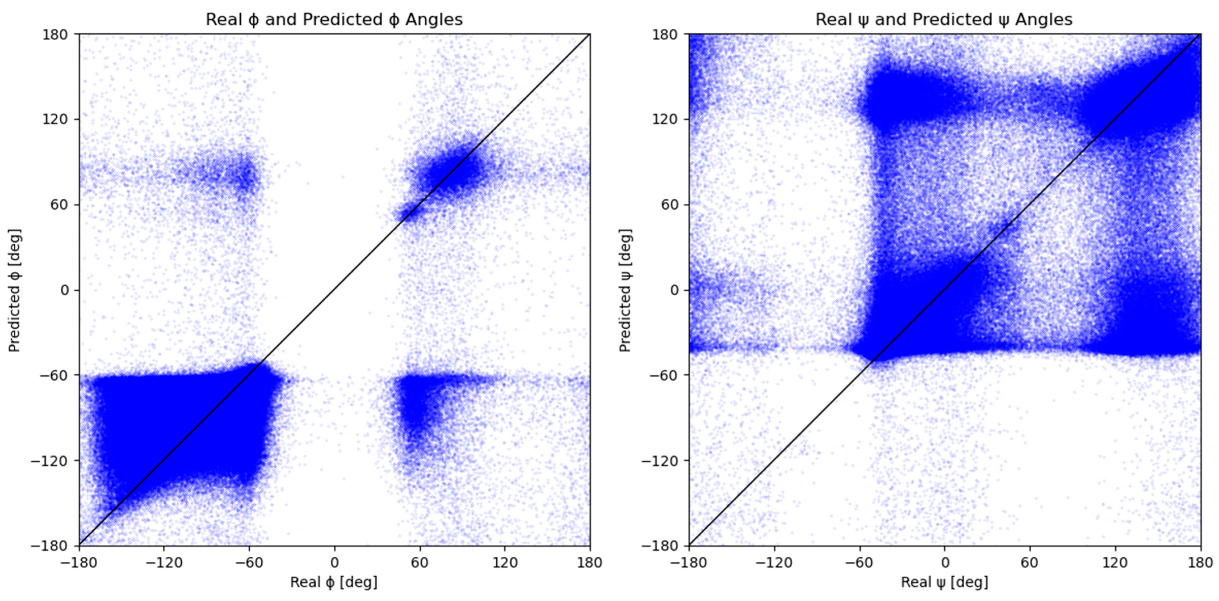
2.2. Measured vs. Predicted Values

The results of Figure 5 show a comparison of measured and predicted dihedral angles, ϕ and ψ. Each blue dot represents a measured-predicted dihedral angle pair. The trend of the distribution of the measured and predicted ϕ and ψ angles from Figure 2 is visible in Figure 5. The graphs in Figure 5 show that the majority of points are divided into two groups that correspond to the major secondary structures and, consequently, to the peaks in Figure 2. Due to the model’s tendency to assign angles that belong to one of the two major secondary structure elements, model predictions result in lower distribution accuracy than individual predictions. This is even more evident from the Figure 5 graph for the ψ dihedral angle since its values are more evenly distributed into two groups.
The discussed groups can be found in Figure 4, located on the graphs’ top left and bottom right edges. A scattered group located around −60° on the x-axis and 70° on the y-axis represents predictions of the ϕ angle that should have been classified as right-handed α-helix, 310-helix, or β-sheet but were instead predicted closer to the left-handed α-helix (Table 1). The other group of mispredicted values is located in the bottom right quadrant, which corresponds to the left-handed α-helix values predicted closer to the right-handed α-helix, 310-helix, or β-sheet in terms of the ϕ angle. An analogous trend can be observed for the graph of measured vs. predicted values of ψ angle, where the resulting scattering is even more prominent due to the existence of two almost equal distributions (Figure 2). Since the peaks of the ψ distribution are almost 180° apart, each mispredicted ψ angle contributes a lot more towards a large MAE than a mispredicted ϕ angle. The Ramachandran plots of the measured and predicted angles (Figure S3) are similar, with well-defined areas for the helices and sheets. The purely predicted Ramachandran plot exhibits higher scattering and a loss of detail when compared to the measured ϕ and ψ angles; however, even a naive one-model prediction can identify general Ramachandran plot trends.

2.3. Dihedral Angle Predictability in Amino Acids

Our model permits an examination of the degree to which adjacent amino acid residues influence the structure of a given amino acid residue and the extent of this influence. To observe this effect, we trained and evaluated the same neural network using a varying sliding window input, ranging from 3 to 21 amino acid residues (Table 2). Our preliminary results indicate that the two closest neighboring residues significantly impact the secondary structure, as shown in Table 2. Interestingly, a sliding window of size three already provides a certain level of accuracy in predicting backbone dihedral angles (28.37 for ϕ and 64.09 for ψ in our tests). However, expanding the sliding window to incorporate 21 residues, with 10 amino acid residues on each side, further enhances the model’s accuracy. These findings align with those reported by Chen K. [50], which stated that the formation of a helical structure can be influenced by amino acids situated up to nine positions away in the sequence. Similarly, the formation of coils and strands can be affected by amino acids up to three and six positions away, respectively, suggesting that for optimal secondary structure prediction, a sliding window comprising 19 residues might be most effective.
Furthermore, regions of the Ramachandran plot previously thought to be conformationally uniform, such as the ones corresponding to α-helices or β-structures, can actually be subdivided based on their distinctive conformational propensities, and these propensities are more influenced by the local (ϕ, ψ) angles than by the secondary structure itself [51]. Comparing our test data with the propensities reported in the literature [52], we observed that both our real and predicted amino acid propensities in the Ramachandran space showcase similarities (Table S2). For instance, residues like Ala, Glu, and Gln exhibit a prominent inclination towards specific alpha-helices, while Val, Thr, and Tyr favor beta-sheets, whereas Gly favors coils.
In supplementary information (Figure S2), we illustrate that Pro ϕ dihedral angles are the most straightforward to predict, whereas predicting ϕ or ψ dihedral angles for Gly proves to be the most challenging. This aligns with the observations in Figure S1, which demonstrates the minimal standard deviation among Pro ϕ dihedral angles and the maximum deviation for Gly ϕ dihedral angles. In general, the prediction of dihedral angles is more complex when they are positioned near the beginning or end of a protein sequence. Yet, this does not seem to significantly affect the ψ dihedral angles of Ile and Val. These angles display an MAE better than 30°—an improvement compared to the average ϕ MAE of 44.14°—across a broad range when they occur at the sequence’s start (up to 10 positions). However, this pattern is not observed when these angles are positioned at the sequence’s end.

2.4. Three-State Secondary Structure Prediction

Although our model was not trained to predict the discrete elements of the protein secondary structure, it can be repurposed by converting the pairs of dihedral angles ϕ and ψ to the three-state secondary structure elements—helix, sheet, and undesignated. Converting the dihedral angles into secondary structure elements is a challenge in itself because most well-known algorithms utilize atomic coordinates to assign secondary structures; however, our dataset is based on a sliding window of residue labels. For example, the STRIDE [53] algorithm recognizes secondary structure elements using hydrogen bond energy and mainchain dihedral angles, while the DSSP of Kasch and Sander [12] employs hydrogen bonds alone. To assign a three-state secondary structure based solely on dihedral angles ϕ and ψ, three areas were determined based on the Ramachandran plot in VMD software (version 1.9.3.) [54] (Figure S4). The secondary structures were then assigned for both measured and predicted dihedral angles of each amino-acid residue from the test dataset. The accuracy of the predicted secondary structures was subsequently determined by comparing the predicted dihedral angles for each residue in the test dataset to the measured dihedral angles. The accuracy was calculated as the number of correctly predicted residues (347 388) divided by the total number of residues (504 024), resulting in an overall accuracy of 68.9% (Table 1).
This study found that our model most accurately predicted sheet structures at a rate of 73.9%, closely followed by helices at 73.2%. However, the prediction accuracy significantly dropped for undesignated structures, which stood at a mere 46.1%. The high accuracy in sheet structure prediction is attributed to their significant representation in the dataset (44.7%; 225,508), facilitating more effective learning of their angle distributions. Conversely, the wide range of dihedral angles from −180° to 180° and their scarce representation in the dataset (16.9%; 85,391) made undesignated structures particularly challenging to predict. One inherent limitation of our analysis is the conversion of continuous dihedral angles into discrete Q3 labels, which may lead to misclassification of predictions at the boundaries of the secondary structure Ramachandran regions. Additionally, the restriction to Q3 rather than Q8 predictions amalgamated all types of helices, potentially counting incorrect dihedral angle predictions as accurate secondary structure elements. We postulate that for our present input data and given the modest model architecture, a naive classification might yield better results than a regression of individual values. Importantly, the improved accuracy in predicting key secondary protein structure components—helices and sheet structures—offers a simplified, yet effective, approach for secondary structure prediction. This capability paves the way for the creation of a foundation, enabling subsequent refinement for more accurate and comprehensive protein structure modeling.
Upon conducting a per-protein analysis on our test dataset, it was observed that the model exhibited a higher degree of accuracy in predicting helices, as evidenced by the MAE values of 15.13° for phi and 36.58° for psi angle, accordingly, pertaining to all-alpha proteins. Conversely, the predictive accuracy for all-beta proteins was found to be lower, potentially due to their underrepresentation in comparison to all-alpha proteins—they constitute merely 25% of the all-alpha protein count.
Moreover, a correlation study was conducted on eleven further experimental systems. These included a small well-described system (PDB ID: 1CRN [55]; Figure S5), a large system of Salinosporamide A complexed with yeast 20S proteasome (PDB ID: 2FAK [56]; Figure S6), homodimeric hemoglobin (PDB ID: 3QOB [57], Figure S7), a medium-sized system E. Coli DNA gyrase subunit B (PDB ID: 4DUH [58]; Figure S8), IFN alpha8 (PDB ID: 6JHD [59]; Figure S9), crystal structure of HL homo-diabody (PDB ID: 6KR0 [60]; Figure S10), a cryo-EM structure of the human PA200 and PA200-20S complex (PDB ID: 6KWY [61]; Figure S11), S109 in complex with CRM1-Ran-RanBP1 (PDB ID: 6LQ9 [62]; Figure S12), and a structure of NHP D11A.F2 Fab (PDB ID: 6XLZ [63]; Figure S13), as well as both Ala and Val MnSOD models (Figures S14 and S15), based on the X-ray diffraction by Azadmanesh, et al. [64] and studied by Broz et al. [65]. All model predictions exhibit MAE values similar to the test dataset predictions, ranging from 12.24°to 28.26° for ϕ errors and from 16.70° to 77.66° for ψ errors (Table S3), and the I model could generally classify the correct secondary structure.

3. Materials and Methods

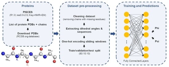
3.1. Dataset Preparation

The dataset was created by extracting proteins from the PISCES [66] database as of February 2023 (Figure S16), which represents a public server for culling sets of protein sequences from the protein data bank (PDB) [67] by sequence identity and structural quality criteria. This database was selected for its ability to provide high-quality lists compared to servers that use BLAST, which often overestimate sequence identity by aligning only well-conserved fragments (alternatives are CoDNas datasets). The criteria used to extract the proteins from PISCES were R-free < 0.25 and protein length ranging from 40 to 10,000 amino acid residues, resulting in a total of 64,220 protein chains. Additional filters were then applied to select models with a resolution of <2.5 Å, one chain per PDB entry, and no missing amino-acid residues, resulting in a final dataset of 20,605 protein chains. To prepare the dataset for analysis, the coordinates of each residue were converted into backbone dihedral angles ϕ and ψ using the Biopython 1.75 Bio.PDB package [68] and Python programming package version 3.10 [69]. The analysis excluded side chains and only considered the first listed amino-acid residue in cases where multiple residues were present due to mutation studies.
Our method employed a sliding window of size 21 for each row of data, which comprises the current amino-acid residue and the 10 residues preceding and following it. This choice was motivated by the trade-off between model accuracy and computational efficiency. As demonstrated in Table 2, while larger window sizes slightly increased accuracy, they also substantially extended the training duration due to the increase in data complexity. At a window size of 21, the accuracy gains practically diminished while computational time escalated.
At the start and end of the protein sequences, where a sliding window of size 21 could not be defined, a virtual amino-acid residue denoted as “0” was introduced. For example, a sliding window of size 21 for a mitochondrial human manganese superoxide dismutase is presented in Figure 6.
In this work, we applied one-hot encoding to the one-letter amino-acid codes using the get_dummies function of the Pandas 1.3.5 library. Each amino-acid residue in the sliding window was encoded into a 20 × 1 vector, yielding 420 independent variables (21 × 20 = 420). Notably, the 21st virtual amino-acid residue we introduced to denote empty spaces at sequence beginnings or ends was represented with a null vector rather than with an additional 20 × 1 vector to optimize computational efficiency. This strategy reduced the potential number of independent variables from 438 to 420 without information loss. The resulting dataset comprised 5,040,244 rows and 422 columns, with the 420 columns representing the one-hot encoded amino-acid residues (the independent variables) and the 2 columns indicating the real ϕ and ψ angles (the dependent variables). This dataset was split into training (80%), validation (10%), and testing (10%) datasets using the train_test_split function in the Tensorflow 2.11.0 package [70].

3.2. Neural Network

In this study, a sequential neural network was utilized to solve a regression problem. The network consisted of an input layer with 420 neurons, four hidden layers with 713 neurons, and an output layer with two neurons (Figure 7). All hidden layers employed the rectified linear unit (ReLU) activation function, while the input and output layers utilized a linear activation function. The network was implemented using the Keras library [71] and Adadelta optimizer [72] with default settings. Network topology was defined and optimized using the Optuna library (https://optuna.org/; accessed on 28 August 2023). In this study, the Adadelta optimizer was selected for training the sequential neural network due to its adaptability, efficiency, and proven success in deep learning, as it forms an adaptive learning rate optimization algorithm that does not require the specification of a fixed learning rate or momentum parameter. The learning rate was set to 0.5, and the training was stopped after four iterations without the validation loss function improvement. The model was trained on four AMD EPYC 7402 24-Core processors.

3.3. Loss Function

The custom loss function was used instead of root mean squared error (RMSE) or MAE because it addresses the periodicity of angles. The function calculates the absolute error for each residue using Equation (1):
AE = min(D, |360 − D|),
where D = |P − A|, P is the predicted angle, and A is the measured angle for an amino-acid residue (Figure 8). This equation ensures that errors near the wrap-around point of 360 degrees are handled appropriately. Namely, due to the periodic nature of angles, the minimum error is 0 degrees and the maximum error is 180 degrees. The mean of these absolute errors is then used as the loss function to train, evaluate, and test the neural network. This approach is consistent with previous studies (SAP [46] and SAP4SS [47]) and is used during all stages of the analysis.

3.4. Optimization

The Bayesian optimization method [73] was constructed using the create_study function in the Optuna hyperparameter optimization framework [74]. While it offers a wealth of sampling and pruning background algorithms, the default settings were used—this encompassed the tree-structured Parzen estimator (TPE) sampler [75] and MedianPruner for pruning. The minimization method was employed to optimize the number of layers and neurons per layer. Bayesian optimization facilitated a more effective exploration of the hyperparameter space through modeling the objective function and employing a probabilistic strategy to maintain a balance between exploration and exploitation during the parameter tuning phase.
The possible hidden layer count was established within a range of one to five, while the neuron count was determined to be between 26 and 840, representing 1/16th and twice the number of the input features, respectively. The optimization procedure, aimed at minimizing the sum of the ϕ and ψ loss functions, was carried out over 30 trials. Figure 9 illustrates that the loss function stopped improving beyond a certain complexity of our neural network. The complexity of a neural network is also directly correlated with the training duration.
In addition to our primary dual-output neural network, we explored potential improvements by optimizing two separate neural networks, each featuring a single output neuron dedicated to predicting either the ϕ or ψ angle. However, as shown in Tables S1–S3, neither approach provided superior accuracy (Figure S17). The two-neuron approach traded off accuracy between the angles, reducing one to minimize the sum of both. Therefore, while either method could be utilized when accuracy is the primary concern, we propose that the dual-output neural network, predicting both angles simultaneously, presents a time-efficient and robust solution. The results can also easily be coupled to further processing steps if needed.

3.5. Predicted Outputs

The neural network has two outputs, representing both ϕ and ψ angles. Hence, only one model was trained for the simultaneous prediction of ϕ and ψ angles. Each pair of ϕ and ψ was associated with one vector with dimensions of 420 × 1, accounting for both angles within one sliding window combination. The angles were managed directly, accommodating their periodicity (−180° to 180°) within the custom loss function of the DNN applied, eliminating the need for using sine and cosine ratios.

4. Conclusions

Our research provides an in-depth analysis of a neural network model that employs a relatively small sliding window in relation to the entire protein length. This approach facilitates our model’s ability to predict dihedral angles without the need for detailed descriptors or the involvement of molecular dynamics simulations. While this streamlined methodology offers clarity in terms of computational understanding, it introduces limitations. Particularly, our model does not effectively capture intra-protein interactions between amino-acid residues located more than ten residues apart, and consequently, it might miss essential molecular interactions such as disulfide bonds, hydrophobic and hydrophilic interactions, hydrogen bonds, and salt bridges.
Despite these challenges, our model represents a perspective application for ab initio structure prediction and the preliminary stages of refinement by providing a basic yet informative representation of the protein backbone structure. Through our evaluations, the model has shown the ability to identify Ramachandran trends and categorize dihedrals into secondary structure elements effectively. While it is not designed to compete directly with advanced, complete folding workflows, its potential within a broader protein folding framework is evident. It is worth noting that many leading protein prediction models integrate multiple simpler models to produce initial structures, which are then refined. Our FCNN model can be envisioned as capable of integrating within such a layered prediction system or being supplemented with additional data to enhance its predictive capabilities.
The central theme of our research has been the exploration of the relationship between model complexity and predictive accuracy. The results from our FCNN model suggest that a model built on a 21-residue primary sequence can achieve notable accuracy in predicting ϕ and ψ dihedral angles. This emphasizes the importance of simplicity in model selection and development—an aspect that sometimes gets overlooked in the current landscape of multi-layered prediction systems. Through our work, we aim to highlight the benefits of balancing performance with computational simplicity. In conclusion, our study encourages the scientific community to reflect on the role of model complexity in determining predictive outcomes. It offers researchers insights into selecting the right model structure and computational approach for their protein folding investigations. In the spirit of open science, our complete work, including the datasets used, is freely available at: https://github.com/maticbroz/phi_psi_prediction_FCNN (accessed on).

Supplementary Materials

The following supporting information can be downloaded at: https://www.mdpi.com/article/10.3390/molecules28207046/s1, Table S1: Exact values of standard deviations of real ϕ and ψ angles in the train and test datasets; Table S2: Real and predicted amino acid conformational propensites of the test dataset; Table S3: Per-model mean absolute errors of the predicted phi and psi dihedral angle of our model com-pared to an online tool DISSpred; Figure S1: A bar graph of standard deviations of real ϕ and ψ angles in the entire dataset by amino-acid residue; Figure S2: Mean absolute error of the current amino-acid residue in relation to the amino-acid residues at different positions of the sliding window for the ϕ (left) and ψ (right) dihedral angles; Figure S3: Ramachandran plots of actual and predicted dihedral angles; Figure S4: Secondary structure areas in the Ramachandran plot. The areas represent secondary structure elements: helices (red), sheets (purple), and undesignated (white). The areas are enclosed by the following points: helix = [(−180.0, −34.9), (−164.3, −42.9), (−133.0, −42.9), (−109.5, −32.2), (−106.9, −21.4), (−44.3, −21.4), (−44.3, −71.1), (−180.0, −71.1)] AND [(62.6, 14.7), (62.6, 96.7), (45.6, 79.2), (45.6, 26.8), (62.6, 14.7)]; sheet = [(−180.2, 42.9), (−140.8, 16.1), (−86.0, 16.1), (−74.3, 45.6), (−74.3, 72.5), (−44.3, 102.0), (−44.3, 161.1), (−46.9, 179.9), (−180, 180)] AND [(−180.0, −163.8), (−75.6, −163.8), (−46.9, −180.0), (−180.0, −180.0)]; Figure S5: Real and predicted ϕ and ψ angles for the protein structure PDB ID: 1CRN (ϕ error = 24.91°; ψ error = 80.86°); Figure S6 Real and predicted ϕ and ψ angles for the protein structure PDB ID: 2FAK (ϕ error = 25.71°; ψ error = 41.96°); Figure S7 Real and predicted ϕ and ψ angles for the protein structure PDB ID: 3QOB (ϕ error = 17.76°; ψ error = 36.43°); Figure S8 Real and predicted ϕ and ψ angles for the protein structure PDB ID: 4DUH (ϕ error = 29.86°; ψ error = 48.16°); Figure S9 Real and predicted ϕ and ψ angles for the protein structure PDB ID: 6JHD (ϕ error = 24.57°; ψ error = 39.91°); Figure S10 Real and predicted ϕ and ψ angles for the protein structure PDB ID: 6KR0 (ϕ error = 12.27°; ψ error = 16.10°); Figure S11 Real and predicted ϕ and ψ angles for the protein structure PDB ID: 6KWY (ϕ error = 22.78°; ψ error = 42.43°); Figure S12 Real and predicted ϕ and ψ angles for the protein structure PDB ID: 6LQ9 (ϕ error = 18.83°; ψ error = 40.67°); Figure S13 Real and predicted ϕ and ψ angles for the protein structure PDB ID: 6XLZ (ϕ error = 17.45°; ψ error = 23.29°); Figure S14 Real and predicted ϕ and ψ angles for the protein structure of MnSOD_ALA (ϕ error = 26.82°; ψ error = 51.12°); Figure S15 Real and predicted ϕ and ψ angles for the protein structure of MnSOD_VAL (ϕ error = 26.41°; ψ error = 50.44°); Figure S16: The process of generating output, which involves accessing the PISCES and RCSB datasets, converting the coordinates to dihedral angles, and transforming the sequence into a sliding window format; Figure S17: Training and validation loss function values during the ϕ and ψ model training.

Author Contributions

Conceptualization, M.B.; methodology, M.B. and M.J.; review and editing, M.B., M.J. and U.B.; original draft preparation, data curation, and visualization, M.B.; supervision and resources, M.J. and U.B. All authors have read and agreed to the published version of the manuscript.

Funding

Financial support through the Slovenian Research Agency program and project grants P2-0046, P1-0403, L2-3175, J1-2471, P2-0438, J4-4633, J1-4398, L2-4430, J3-4498, J7-4638, J1-4414, I0-E015, J1-50034, J7-50043 and J3-4497 is gratefully acknowledged. We thank OpenEye (https://www.eyesopen.com, accessed on 10 October 2023) for the academic licensing of their software and their support. The authors gratefully acknowledge the HPC RIVR consortium (www.hpc-rivr.si, accessed on 5 November 2022) for providing computational resources for the HPC systems VEGA and MAISTER at the University of Maribor (www.um.si, accessed on 10 October 2023).

Institutional Review Board Statement

Not applicable.

Informed Consent Statement

Not applicable.

Data Availability Statement

All data is contained within the article, supplementary material, and the provided GitHub repository.

Conflicts of Interest

The authors declare no conflict of interest.

Sample Availability

Not applicable.

Abbreviations

7PCP7 physicochemical properties
AMDAdvanced Micro Devices
ASAaccessible surface area
Bisolated β-bridge
BAPprotein backbone angle predictions
BLASTBasic Local Alignment Search Tool
BRNNbidirectional recurrent neural network
Ccarbon atom ooil
CASPCritical Assessment of protein Structure Prediction
CNNconvolutional neural network
CoDNasConformational Diversity of Native State
alpha carbon atom
DNNdeep neural network
Eparallel/anti-parallel β sheet conformation
Esheet
FCNNfully connected neural network
FMfree modeling
G310 helix
Hα-helix
HHBlitsHMM-HMM-based lightning-fast iterative sequence search
HMMhidden Markov model
Iπ-helix
LSTMlong short-term memory
LSTM-BRNNslong short-term memory and bidirectional recurrent neural networks
MAEmean absolute error
MDmolecular dynamics
MTSmitoargetingtargetting sequence
MnSODmanganese superoxide dismutase
Nnitrogen atom
PDBProtein Data Bank
PISCESProtein sequence culling server
PSPprotein structure prediction
PSSMposition-specific scoring matrix
PSSPprotein secondary structure prediction
Q3three-state model
Q8eight-state model
R-freeFree R-value
RMSEroot mean squared error
ReLURectified Linear Unit
ResNetsResidual Networks
ResNetsresidual networks
Sbend
SAPstructure analysis and prediction
SNPsingle nucleotide polymorphism
SSsecondary structure
SSProSecondary Structure Prediction
SVMsupport vector machine
Tturn
ÅAngstrom
τtao
ψpsi dihedral angle
ωomega dihedral angle
ϕphi dihedral angle

References

  1. Cutello, V.; Narzisi, G.; Nicosia, G. A multi-objective evolutionary approach to the protein structure prediction problem. J. R. Soc. Interface 2005, 3, 139–151. [Google Scholar] [CrossRef] [PubMed]
  2. Jumper, J.; Evans, R.; Pritzel, A.; Green, T.; Figurnov, M.; Ronneberger, O.; Tunyasuvunakool, K.; Bates, R.; Žídek, A.; Potapenko, A.; et al. Highly accurate protein structure prediction with AlphaFold. Nature 2021, 596, 583–589. [Google Scholar] [CrossRef] [PubMed]
  3. AlQuraishi, M. AlphaFold at CASP13. Bioinformatics 2019, 35, 4862–4865. [Google Scholar] [CrossRef] [PubMed]
  4. Kryshtafovych, A.; Schwede, T.; Topf, M.; Fidelis, K.; Moult, J. Critical assessment of methods of protein structure prediction (CASP)-round XIII. Proteins 2019, 87, 1011–1020. [Google Scholar] [CrossRef] [PubMed]
  5. Pereira, J.; Simpkin, A.J.; Hartmann, M.D.; Rigden, D.J.; Keegan, R.M.; Lupas, A.N. High-accuracy protein structure prediction in CASP14. Proteins 2021, 89, 1687–1699. [Google Scholar] [CrossRef] [PubMed]
  6. Senior, A.W.; Evans, R.; Jumper, J.; Kirkpatrick, J.; Sifre, L.; Green, T.; Qin, C.; Žídek, A.; Nelson, A.W.R.; Bridgland, A.; et al. Improved protein structure prediction using potentials from deep learning. Nature 2020, 577, 706–710. [Google Scholar] [CrossRef] [PubMed]
  7. Guo, J.-T.; Ellrott, K.; Xu, Y. A historical perspective of template-based protein structure prediction. In Protein Structure Prediction; Humana: Totowa, NJ, USA, 2008; pp. 3–42. [Google Scholar]
  8. Zhou, Y.; Duan, Y.; Yang, Y.; Faraggi, E.; Lei, H. Trends in template/fragment-free protein structure prediction. Theor. Chem. Acc. 2011, 128, 3–16. [Google Scholar] [CrossRef]
  9. Maurice, K.J. SSThread: Template-free protein structure prediction by threading pairs of contacting secondary structures followed by assembly of overlapping pairs. J. Comput. Chem. 2014, 35, 644–656. [Google Scholar] [CrossRef]
  10. Rost, B. Protein secondary structure prediction continues to rise. J. Struct. Biol. 2001, 134, 204–218. [Google Scholar] [CrossRef]
  11. Pauling, L.; Corey, R.B.; Branson, H.R. The structure of proteins: Two hydrogen-bonded helical configurations of the polypeptide chain. Proc. Natl. Acad. Sci. USA 1951, 37, 205–211. [Google Scholar] [CrossRef]
  12. Kabsch, W.; Sander, C. Dictionary of protein secondary structure: Pattern recognition of hydrogen-bonded and geometrical features. Biopolymers 1983, 22, 2577–2637. [Google Scholar] [CrossRef] [PubMed]
  13. Nagy, G.; Oostenbrink, C. Dihedral-based segment identification and classification of biopolymers I: Proteins. J. Chem. Inf. Model. 2014, 54, 266–277. [Google Scholar] [CrossRef] [PubMed]
  14. Rost, B.; Sander, C. Prediction of protein secondary structure at better than 70% accuracy. J. Mol. Biol. 1993, 232, 584–599. [Google Scholar] [CrossRef] [PubMed]
  15. Jones, D.T. Protein secondary structure prediction based on position-specific scoring matrices. J. Mol. Biol. 1999, 292, 195–202. [Google Scholar] [CrossRef] [PubMed]
  16. Dor, O.; Zhou, Y. Achieving 80% ten-fold cross-validated accuracy for secondary structure prediction by large-scale training. Proteins 2007, 66, 838–845. [Google Scholar] [CrossRef] [PubMed]
  17. Faraggi, E.; Zhang, T.; Yang, Y.; Kurgan, L.; Zhou, Y. SPINE X: Improving protein secondary structure prediction by multistep learning coupled with prediction of solvent accessible surface area and backbone torsion angles. J. Comput. Chem. 2012, 33, 259–267. [Google Scholar] [CrossRef] [PubMed]
  18. Bettella, F.; Rasinski, D.; Knapp, E.W. Protein secondary structure prediction with SPARROW. J. Chem. Inf. Model. 2012, 52, 545–556. [Google Scholar] [CrossRef] [PubMed]
  19. Mirabello, C.; Pollastri, G. Porter, PaleAle 4.0: High-accuracy prediction of protein secondary structure and relative solvent accessibility. Bioinformatics 2013, 29, 2056–2058. [Google Scholar] [CrossRef]
  20. Yaseen, A.; Li, Y. Context-based features enhance protein secondary structure prediction accuracy. J. Chem. Inf. Model. 2014, 54, 992–1002. [Google Scholar] [CrossRef]
  21. Heffernan, R.; Paliwal, K.; Lyons, J.; Dehzangi, A.; Sharma, A.; Wang, J.; Sattar, A.; Yang, Y.; Zhou, Y. Improving prediction of secondary structure, local backbone angles, and solvent accessibility with a single neural network. Sci. Rep. 2015, 83, 1201–1214. [Google Scholar]
  22. Cuff, J.A.; Barton, G.J. Application of multiple sequence alignment profiles to improve protein secondary structure prediction. Proteins 2000, 40, 502–511. [Google Scholar] [CrossRef]
  23. Drozdetskiy, A.; Cole, C.; Procter, J.; Barton, G.J. JPred4: A protein secondary structure prediction server. Nucleic Acids Res. 2015, 43, W389–W394. [Google Scholar] [CrossRef] [PubMed]
  24. Wang, S.; Peng, J.; Ma, J.; Xu, J. Protein secondary structure prediction using deep convolutional neural fields. Sci. Rep. 2016, 6, 18962. [Google Scholar] [CrossRef] [PubMed]
  25. Heffernan, R.; Yang, Y.; Paliwal, K.; Zhou, Y. Capturing non-local interactions by long short-term memory bidirectional recurrent neural networks for improving prediction of protein secondary structure, backbone angles, contact numbers, and solvent accessibility. Bioinformatics 2017, 33, 2842–2849. [Google Scholar] [CrossRef] [PubMed]
  26. Fang, C.; Shang, Y.; Xu, D. MUFOLD-SS: New deep inception-inside-inception networks for protein secondary structure prediction. Proteins 2018, 86, 592–598. [Google Scholar] [CrossRef] [PubMed]
  27. Klausen, M.S.; Jespersen, M.C.; Nielsen, H.; Jensen, K.K.; Jurtz, V.I.; Sønderby, C.K.; Sommer, M.O.A.; Winther, O.; Nielsen, M.; Petersen, B.; et al. NetSurfP-2.0: Improved prediction of protein structural features by integrated deep learning. Proteins Struct. Funct. Bioinform. 2019, 87, 520–527. [Google Scholar] [CrossRef] [PubMed]
  28. Zhang, B.; Li, J.; Lü, Q. Prediction of 8-state protein secondary structures by a novel deep learning architecture. BMC Bioinform. 2018, 19, 293. [Google Scholar] [CrossRef] [PubMed]
  29. Xu, G.; Wang, Q.; Ma, J. OPUS-TASS: A protein backbone torsion angles and secondary structure predictor based on ensemble neural networks. Bioinformatics 2020, 36, 5021–5026. [Google Scholar] [CrossRef] [PubMed]
  30. Guo, Z.; Hou, J.; Cheng, J. DNSS2: Improved ab initio protein secondary structure prediction using advanced deep learning architectures. Proteins 2021, 89, 207–217. [Google Scholar] [CrossRef]
  31. Pollastri, G.; Przybylski, D.; Rost, B.; Baldi, P. Improving the prediction of protein secondary structure in three and eight classes using recurrent neural networks and profiles. Proteins 2002, 47, 228–235. [Google Scholar] [CrossRef]
  32. Wang, Z.; Zhao, F.; Peng, J.; Xu, J. Protein 8-class secondary structure prediction using conditional neural fields. Proteomics 2011, 11, 3786–3792. [Google Scholar] [CrossRef] [PubMed]
  33. Yaseen, A.; Li, Y. Template-based C8-SCORPION: A protein 8-state secondary structure prediction method using structural information and context-based features. Bioinformatics 2014, 15, S3. [Google Scholar] [CrossRef] [PubMed]
  34. Zhou, J.; Troyanskaya, O.G. Deep supervised and convolutional generative stochastic network for protein secondary structure prediction. In Proceedings of the 31st International Conference on International Conference on Machine Learning, Beijing, China, 21–26 June 2014. [Google Scholar]
  35. Simons, K.T.; Kooperberg, C.; Huang, E.; Baker, D.; Petrey, D. Improved recognition of native-like protein structures using a combination of sequence-dependent and sequence-independent features of proteins. Proteins Struct. Funct. Bioinform. 1999, 34, 82–95. [Google Scholar] [CrossRef]
  36. Faraggi, E.; Yang, Y.; Zhang, S.; Zhou, Y. Predicting continuous local structure and the effect of its substitution for secondary structure in fragment-free protein structure prediction. Structure 2009, 17, 1515–1527. [Google Scholar] [CrossRef] [PubMed]
  37. Lyons, J.; Dehzangi, A.; Heffernan, R.; Sharma, A.; Paliwal, K.; Sattar, A.; Zhou, Y.; Yang, Y. Predicting backbone cα angles and dihedrals from protein sequences by stacked sparse auto-encoder deep neural network. J. Comput. Chem. 2014, 35, 2040–2046. [Google Scholar] [CrossRef] [PubMed]
  38. Hanson, J.; Paliwal, K.; Litfin, T.; Yang, Y.; Zhou, Y. Improving prediction of protein secondary structure, backbone angles, solvent accessibility and contact numbers by using predicted contact maps and an ensemble of recurrent and residual convolutional neural networks. Bioinformatics 2018, 35, 2403–2410. [Google Scholar] [CrossRef] [PubMed]
  39. Altschul, S.F.; Madden, T.L.; Schäffer, A.A.; Zhang, J.; Zhang, Z.; Miller, W.; Lipman, D.J. Gapped BLAST and PSI-BLAST: A new generation of protein database search programs. Nucleic Acids Res. 1997, 25, 3389–3402. [Google Scholar] [CrossRef] [PubMed]
  40. Fang, C. Applications of Deep Neural Networks to Protein Structure Prediction. Ph.D. Thesis, University of Missouri, Columbia, MO, USA, 2018. [Google Scholar]
  41. Wu, S.; Zhang, Y. Anglor: A composite machine-learning algorithm for protein backbone torsion angle prediction. PLoS ONE 2008, 3, e3400. [Google Scholar] [CrossRef]
  42. Remmert, M.; Biegert, A.; Hauser, A.; Söding, J. HHblits: Lightning-fast iterative protein sequence searching by hmm-hmm alignment. Nat. Methods 2012, 9, 173. [Google Scholar] [CrossRef]
  43. Heffernan, R.; Paliwal, K.; Lyons, J.; Singh, J.; Yang, Y.; Zhou, Y. Single-sequence-based prediction of protein secondary structures and solvent accessibility by deep whole-sequence learning. J. Comput. Chem. 2018, 39, 2210–2216. [Google Scholar] [CrossRef]
  44. Hanson, J.; Paliwal, K.; Litfin, T.; Yang, Y.; Zhou, Y. Accurate prediction of protein contact maps by coupling residual two-dimensional bidirectional long short-term memory with convolutional neural networks. Bioinformatics 2018, 34, 4039–4045. [Google Scholar] [CrossRef] [PubMed]
  45. Gao, Y.; Wang, S.; Deng, M.; Xu, J. Raptorx-angle: Real-value prediction of protein backbone dihedral angles through a hybrid method of clustering and deep learning. Bioinformatics 2018, 19, 73–84. [Google Scholar] [CrossRef] [PubMed]
  46. Mataeimoghadam, F.; Hakim Newton, M.A.; Dehzangi, A.; Karim, A.; Jayaram, B.; Ranganathan, S.; Sattar, A. Enhancing protein backbone angle prediction by using simpler models of deep neural networks. Sci. Rep. 2020, 10, 5016. [Google Scholar] [CrossRef] [PubMed]
  47. Newton, M.A.H.; Mataeimoghadam, F.; Zaman, R.; Sattar, A. Secondary structure specific simpler prediction models for protein backbone angles. Bioinformatics 2022, 23, 6. [Google Scholar] [CrossRef] [PubMed]
  48. McKinney, W. Data structures for statistical computing in python. In Proceedings of the 9th Python in Science Conference, Austin, TX, USA, 28 June–3 July 2010; Volume 445, pp. 51–56. [Google Scholar]
  49. Hunter, J.D. Matplotlib: A 2D graphics environment. Comput. Sci. Eng. 2007, 9, 90–95. [Google Scholar] [CrossRef]
  50. Chen, K.; Kurgan, L.; Ruan, J. Optimization of the Sliding Window Size for Protein Structure Prediction. In Proceedings of the IEEE Symposium on Computational Intelligence and Bioinformatics and Computational Biology, Toronto, ON, Canada, 28–29 September 2006; pp. 1–7. [Google Scholar]
  51. Balasco, N.; Esposito, L.; De Simone, A.; Vitagliano, L. Local Backbone Geometry Plays a Critical Role in Determining Conformational Preferences of Amino Acid Residues in Proteins. Biomolecules 2022, 12, 1184. [Google Scholar] [CrossRef] [PubMed]
  52. Swindells, M.B.; MacArthur, M.W.; Thornton, J.M. Intrinsic φ,ψ propensities of amino acids, derived from the coil regions of known structures. Nat. Struct. Mol. Biol. 1995, 2, 596–603. [Google Scholar] [CrossRef]
  53. Heinig, M.; Frishman, D. STRIDE: A Web server for secondary structure assignment from known atomic coordinates of proteins. Nucleic Acids Res. 2004, 32, W500–W502. [Google Scholar] [CrossRef]
  54. Humphrey, W.; Dalke, A.; Schulten, K. VMD—Visual Molecular Dynamics. J. Molec. Graph. 1996, 14, 33–38. [Google Scholar] [CrossRef]
  55. Teeter, M.M. Water structure of a hydrophobic protein at atomic resolution: Pentagon rings of water molecules in crystals of crambin. Proc. Natl. Acad. Sci. USA 1984, 81, 6014–6018. [Google Scholar] [CrossRef]
  56. Groll, M.; Huber, R.; Potts, B.C. Crystal structures of Salinosporamide A (NPI-0052) and B (NPI-0047) in complex with the 20S proteasome reveal important consequences of beta-lactone ring opening and a mechanism for irreversible binding. J. Am. Chem. Soc. 2006, 128, 5136–5141. [Google Scholar] [CrossRef] [PubMed]
  57. Ren, Z.; Srajer, V.; Knapp, J.E.; Royer, W.E., Jr. Cooperative macromolecular device revealed by meta-analysis of static and time-resolved structures. Proc. Natl. Acad. Sci. USA 2012, 109, 107–112. [Google Scholar] [CrossRef] [PubMed]
  58. Brvar, M.; Perdih, A.; Renko, M.; Anderluh, G.; Turk, D.; Solmajer, T. Structure-based discovery of subst’tuted 4,5’-bithiazoles as novel DNA gyrase inhibitors. J. Med. Chem. 2012, 55, 6413–6426. [Google Scholar] [CrossRef] [PubMed]
  59. Ken-ichi, A.; Shigeyuki, M. Solution Structure of IFN alpha8. Available online: https://www.rcsb.org/structure/6jhd (accessed on 3 October 2023).
  60. Nakazawa, H.; Onodera-Sugano, T.; Sugiyama, A.; Tanaka, Y.; Hattori, T.; Niide, T.; Ogata, H.; Asano, R.; Kumagai, I.; Umetsu, M. Association behavior and control of the quality of cancer therapeutic bispecific diabodies expressed in Escherichia coli. Biochem. Eng. J. 2020, 160, 107636. [Google Scholar] [CrossRef]
  61. Guan, H.; Wang, Y.; Yu, T.; Huang, Y.; Li, M.; Saeed, A.F.U.H.; Perčulija, V.; Li, D.; Xiao, J.; Wang, D.; et al. Cryo-EM structures of the human PA200 and PA200-20S complex reveal regulation of proteasome gate opening and two PA200 apertures. PLoS Biol. 2020, 18, e3000654. [Google Scholar] [CrossRef] [PubMed]
  62. Lei, Y.; An, Q.; Shen, X.F.; Sui, M.; Li, C.; Jia, D.; Luo, Y.; Sun, Q. Structure-Guided Design of the First Noncovalent Small-Molecule Inhibitor of CRM1. J. Med. Chem. 2021, 64, 6596–6607. [Google Scholar] [CrossRef] [PubMed]
  63. Aljedani, S.S.; Liban, T.J.; Tran, K.; Phad, G.; Singh, S.; Dubrovskaya, V.; Pushparaj, P.; Martinez-Murillo, P.; Rodarte, J.; Mileant, A.; et al. Structurally related but genetically unrelated antibody lineages converge on an immunodominant HIV-1 Env neutralizing determinant following trimer immunization. PLoS Pathog. 2021, 17, e1009543. [Google Scholar] [CrossRef] [PubMed]
  64. Azadmanesh, J.; Trickel, S.R.; Borgstahl, G.E.O. Substrate-analog binding and electrostatic surfaces of human manganese superoxide dismutase. J. Struct. Biol. 2017, 199, 68–75. [Google Scholar] [CrossRef]
  65. Broz, M.; Furlan, V.; Lešnik, S.; Jukič, M.; Bren, U. The Effect of the Ala16Val Mutation on the Secondary Structure of the Manganese Superoxide Dismutase Mitochondrial Targeting Sequence. Antioxidants 2022, 11, 2348. [Google Scholar] [CrossRef]
  66. Wang, G.; Dunbrack, R.L., Jr. PISCES: A protein sequence culling server. Bioinformatics 2003, 19, 1589–1591. [Google Scholar] [CrossRef]
  67. Berman, H.M.; Westbrook, J.; Feng, Z.; Gilliland, G.; Bhat, T.N.; Weissig, H.; Shindyalov, I.N.; Bourne, P.E. The Protein Data Bank. Nucleic Acids Res. 2000, 28, 235–242. [Google Scholar] [CrossRef]
  68. Cock, P.J.; Antao, T.; Chang, J.T.; Chapman, B.A.; Cox, C.J.; Dalke, A.; Friedberg, I.; Hamelryck, T.; Kauff, F.; Wilczynski, B.; et al. Biopython: Freely available Python tools for computational molecular biology and bioinformatics. Bioinformatics 2009, 25, 1422–1423. [Google Scholar] [CrossRef]
  69. Van Rossum, G.; Drake, F.L. Python 3 Reference Manual; CreateSpace: Scotts Valley, CA, USA, 2009. [Google Scholar]
  70. Abadi, M.; Barham, P.; Chen, J.; Chen, Z.; Davis, A.; Dean, J.; Devin, M.; Ghemawat, S.; Irving, G.; Isard, M.; et al. TensorFlow: A system for large-scale machine learning. In Proceedings of the 12th USENIX Symposium on Operating Systems Design and Implementation (OSDI 16), Savannah, GA, USA, 2–4 November 2016; pp. 265–283. [Google Scholar]
  71. Chollet, F.; Keras. GitHub. Available online: https://github.com/fchollet/keras (accessed on 12 February 2022).
  72. Zeiler, M.D. ADADELTA: An Adaptive Learning Rate Method. arXiv 2012, arXiv:1212.5701. [Google Scholar]
  73. Močkus, J. Bayesian Approach to Global Optimization. Mathematics and Its Applications, 37th ed.; Kluwer Academic Publishers Group: Dordrecht, The Netherlands, 1989; ISBN 978-94-009-0909-0. [Google Scholar]
  74. Takuya, A.; Shotaro, S.; Yanase, T.; Ohta, T. Optuna: A Next-generation Hyperparameter Optimization Framework. In Proceedings of the 25th ACM SIGKDD International Conference on Knowledge Discovery & Data Mining, New York, NY, USA, 4–8 August 2009; pp. 2623–2631. [Google Scholar]
  75. Bergstra, J.; Bardenet, R.; Bengio, Y.; Kégl, B. Algorithms for Hyper-Parameter Optimization. In Proceedings of the 24th International Conference on Neural Information Processing Systems, Granada, Spain, 12–14 December 2011; pp. 2546–2554. [Google Scholar]
Figure 1. A schematic representation of ϕ, ψ, and ω protein backbone dihedral angles. Grey spheres represent carbon atoms, blue spheres nitrogen atoms, and red spheres oxygen atoms.
Molecules 28 07046 g001
Figure 2. Distribution of measured angles of the testing dataset and neural network predictions. The blue lines represent the measured ϕ and ψ angle distributions of the test dataset, while the orange lines represent the neural network-predicted ϕ and ψ angle distributions of the test dataset.
Molecules 28 07046 g002
Figure 3. Mean absolute prediction error per amino-acid residue. A mean absolute prediction error and its standard deviation were calculated for each amino-acid residue for ϕ (blue) and ψ (orange) dihedral angles.
Molecules 28 07046 g003
Figure 4. Distribution of the absolute angle prediction errors for ϕ and ψ with a resolution of 1 degree.
Molecules 28 07046 g004
Figure 5. Predicted dihedral angles in relation to the measured dihedral angles. Each blue dot represents one set of measured and predicted ϕ and ψ dihedral angles. The black y = x line represents the ideal distribution, where each predicted angle is equal to its measured counterpart.
Molecules 28 07046 g005
Figure 6. A schematic representation of the amino-acid residue sliding window, using the FASTA sequence of the 5VF9 [64] model. The sliding window consists of 10 amino-acid residues before and 10 amino-acid residues after the current amino-acid residue, shifting the window by one amino-acid residue to the right at each step. Virtual residues denoted by “0” were added to the start and end of the sequence to define the sliding window in these regions. The current amino-acid residue is indicated with a bold letter, while the sliding window is highlighted in light blue.
Molecules 28 07046 g006
Figure 7. The structure of the applied neural network. The gray circles symbolize individual neurons, while the arrows indicate connections from the output of one artificial neuron to the input of another. This network consists of four hidden layers, with the input layer containing 420 neurons, all four hidden layers 713 neurons each, and the output layer 2 neurons. All layers, except the last one, utilize the ReLU activation function.
Molecules 28 07046 g007
Figure 8. The schematic representation of the custom loss function. For illustrative purposes, the real angle is set at 0 degrees, while the predicted angle is 245 degrees. In this case, D is 245°, while |360° − D| is 115°. The custom loss function adopts the minimum value between D and |360° − D|, which in this instance is 115°. This methodology ensures that all calculated errors are confined within the appropriate range of [0, 180°].
Molecules 28 07046 g008
Figure 9. Total loss function (ϕ + ψ) in relation to the number of parameters of the neural network. The total number of parameters in a sequential neural network was calculated by adding the product of the number of neurons in each layer with the number of neurons in the following layer for all layers. This represents the total number of connection weights between neurons in adjacent layers, which yields a single number indicative of the network’s size and complexity.
Molecules 28 07046 g009
Table 1. The portion of the real helix, sheet, and undesignated secondary structures predicted as either helix, sheet, or undesignated secondary structures.
SS LabelHelix (Predicted)Sheet (Predicted)Undesignated (Predicted)
Helix (real)73.2% (141,380)16.0% (30,837)10.8% (20,908)
Sheet (real)14.9% (33,535)73.9% (166,673)11.2% (25,300)
Undesignated (real)27.1% (23,151)26.8% (22,905)46.1% (39,335)
Table 2. The correlation between the sliding window size, the accuracy of the model, and the training duration.
Sliding WindowPhi MAE [deg]Psi MAE [deg]Epoch Duration [s]
328.3764.0957
725.6753.36102
1124.5148.98130
1523.9646.74155
2123.5344.14210
Disclaimer/Publisher’s Note: The statements, opinions and data contained in all publications are solely those of the individual author(s) and contributor(s) and not of MDPI and/or the editor(s). MDPI and/or the editor(s) disclaim responsibility for any injury to people or property resulting from any ideas, methods, instructions or products referred to in the content.

