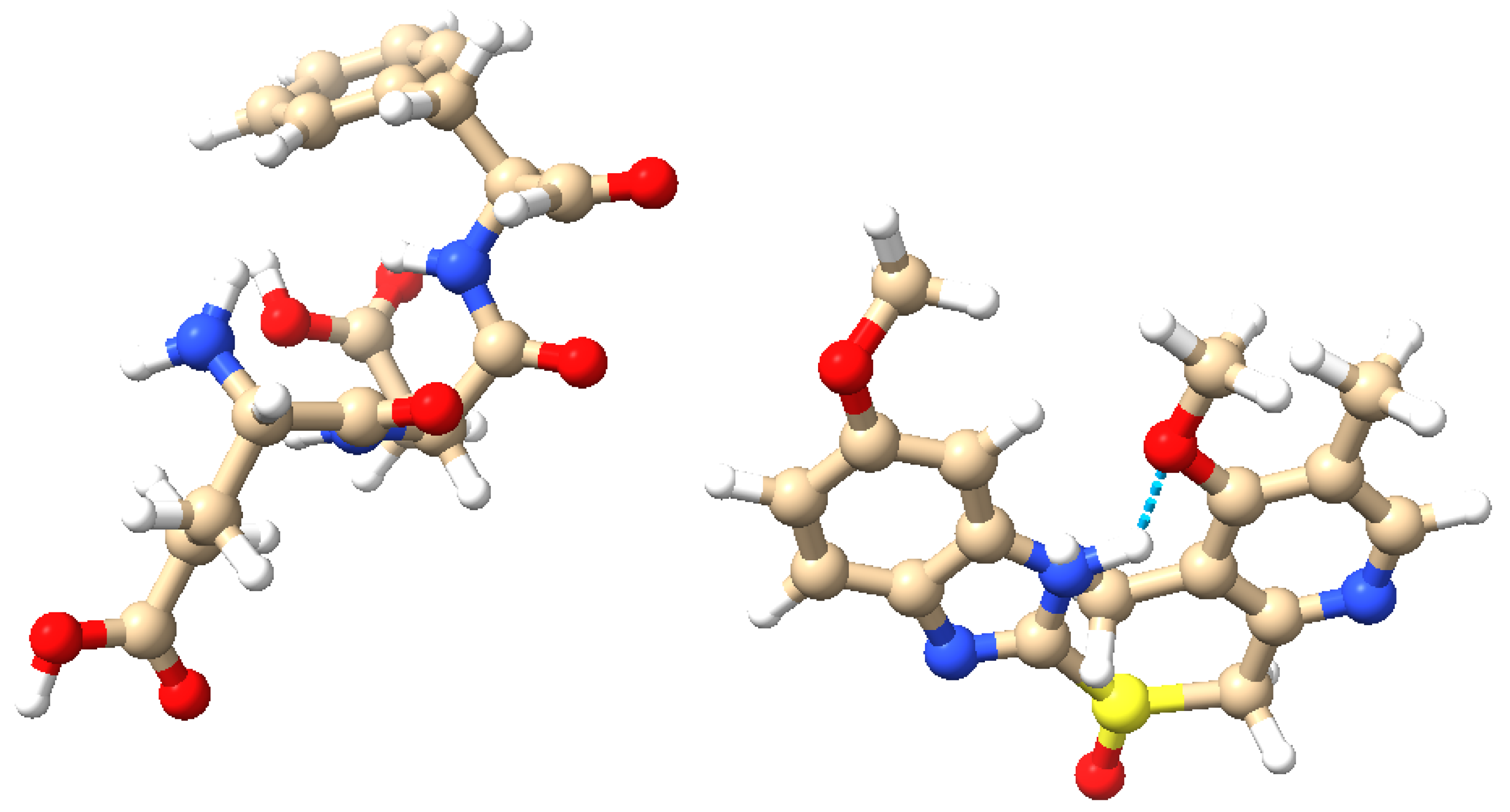
Figure 1.
Molecular structures of the proteinoid and omeprazole. (
Left): The proteinoid composed of L-glutamic acid (L-Glu), L-aspartic acid (L-Asp), and L-phenylalanine (L-Phe). (
Right): The omeprazole molecule. Atoms are colour-coded: blue (nitrogen), red (oxygen), brown (carbon), yellow (sulphur), and white (hydrogen). Potential hydrogen bonding is highlighted, illustrating the possible interactions between the proteinoid and omeprazole. These molecular structures and their interactions are key to understanding the complex signal processing behaviour observed in the omeprazole–proteinoid system. (visualisation created using UCSF Chimera [
21]).
Figure 2.
A conceptual diagram illustrating the unconventional computing strategy involving omeprazole–proteinoid complexes and Izhikevich neuron models. The graphic depicts the combination of chemical components (shown by ellipses) with computational components (represented by rectangles) to regulate different neural behaviours.
Figure 3.
Diagram illustrating the setup used for the electrochemical characterisation of the proteinoid solution, with and without omeprazole. The solution is contained within the central container, equipped with two needle electrodes coated with platinum (Pt) and iridium (Ir), respectively, positioned 10 mm apart. A high-precision 24-bit ADC data recorder captures voltage responses between these electrodes. A heating block regulates temperature. A function generator produces stimuli that simulate neuron-like membrane potential changes, applied between the electrodes. This setup allows for the identification of very small voltage changes (in the microvolts range) and the analysis of the spatial and temporal patterns of voltage responses in the proteinoid solution. Control experiments are conducted using the same setup with different chemicals to isolate the specific effects of omeprazole.
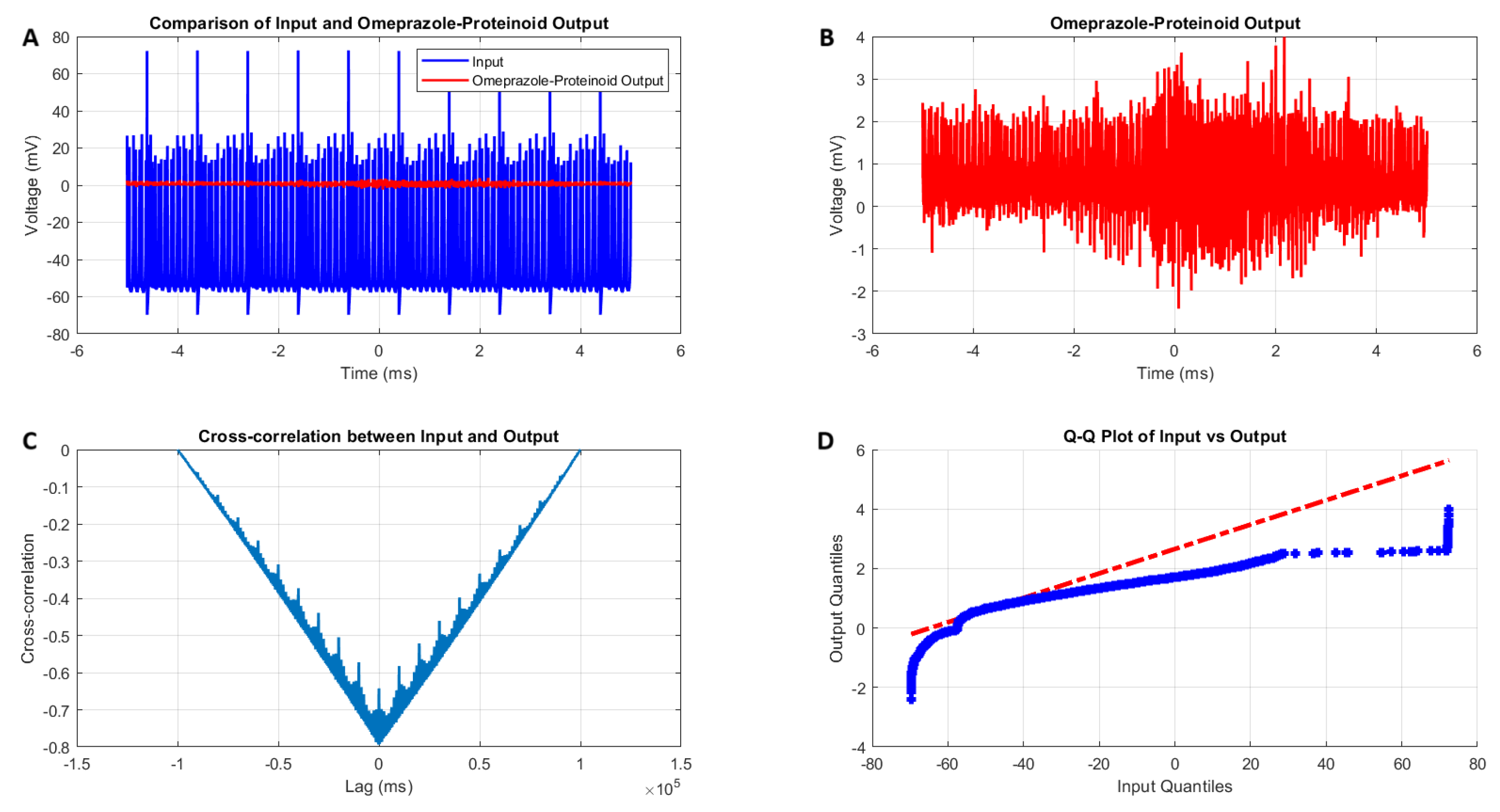
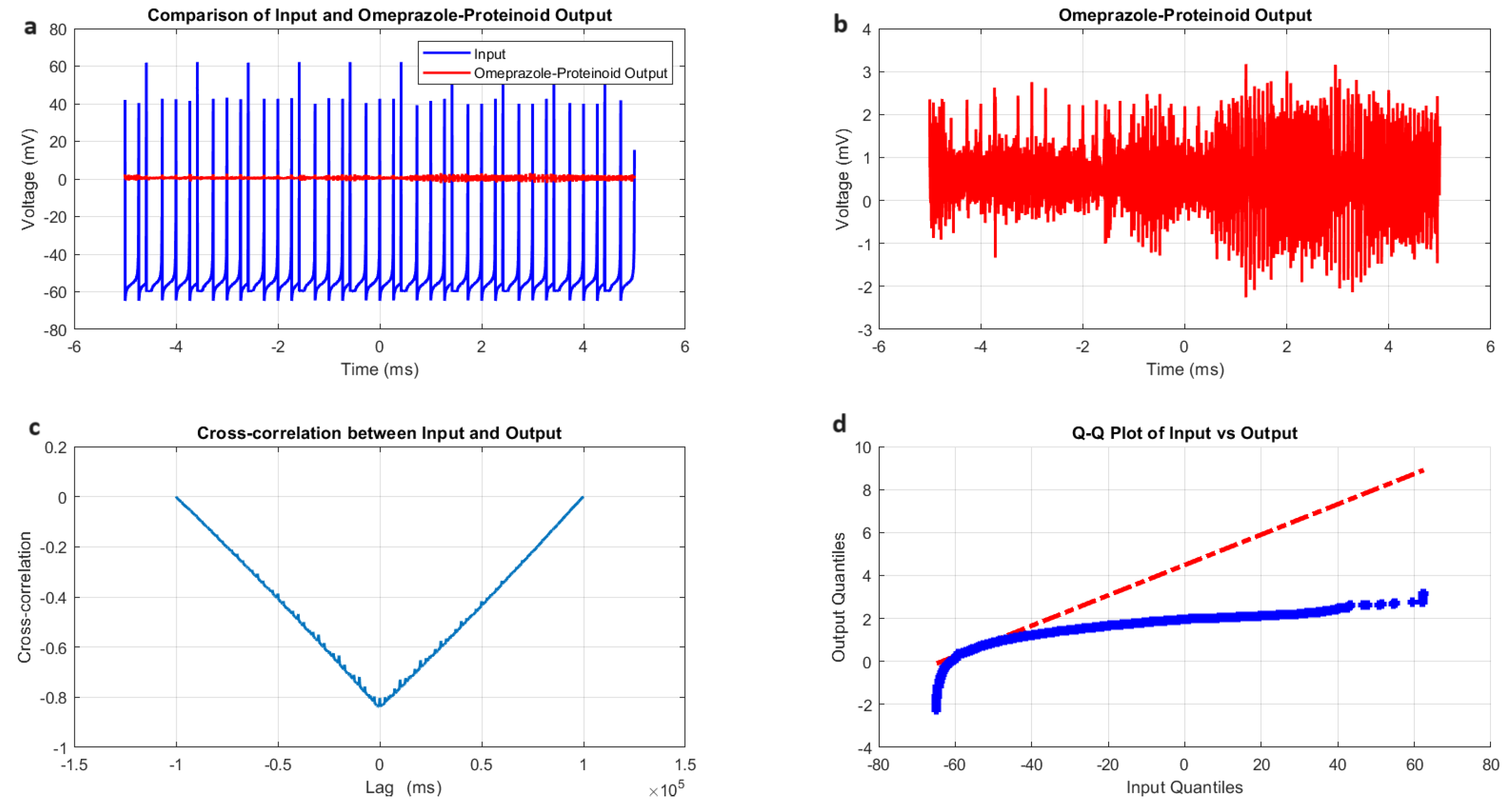
Figure 4.
Analysis of the Izhikevich neuron accommodation spiking and omeprazole–proteinoid complex interaction. (A) Comparison of the input Izhikevich neuron signal (blue, range: to 72.50 mV) and omeprazole–proteinoid output (red, range: to 3.99 mV), showing significant amplitude attenuation. (B) Isolated omeprazole–proteinoid output, revealing subtle voltage fluctuations (mean: 0.60 mV, SD: 0.43 mV) in response to input. (C) Cross-correlation between input and output, indicating a time lag of ms and a moderate positive correlation (r = 0.6841). (D) The blue dots represent the data points, while the red dashed line represents the theoretical line for a normal distribution. Q-Q plot demonstrating substantial deviation from the identity line, confirming significantly different distributions (Kolmogorov–Smirnov test: p < 0.0001, KS statistic: 0.9709). The omeprazole–proteinoid complex exhibits a marked filtering effect, reducing signal amplitude while preserving some temporal characteristics of the input. The RMSE of 50.4592 mV and maximum difference of 71.92 mV (at 1.39 ms) further quantify the substantial transformation of the signal. This analysis suggests the complex neuromodulatory effects of the omeprazole–proteinoid interaction on the accommodation spiking patterns.
![Molecules 29 04700 g004]()
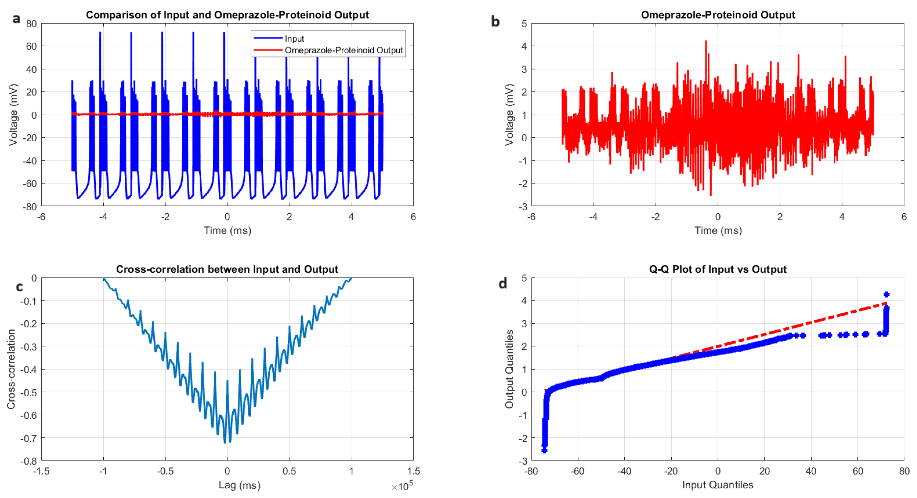
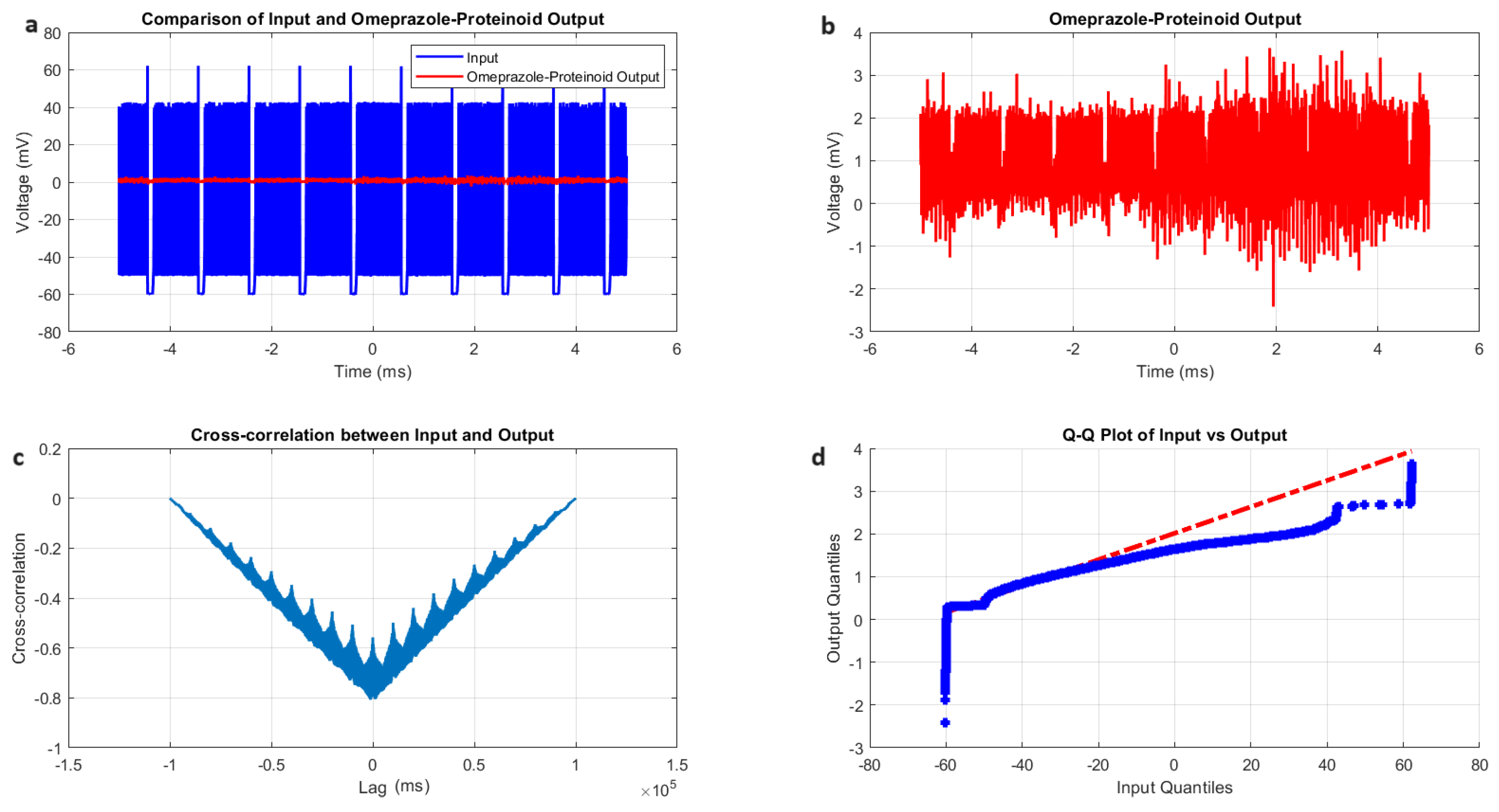
Figure 5.
Chattering spiking stimulation analysis of omeprazole–proteinoid sample. (a) Input–output comparison showing the input signal (mean: mV, SD: 19.72 mV) and the omeprazole–proteinoid output (mean: 0.48 mV, SD: 0.51 mV). Correlation coefficient: 0.7937, RMSE: 59.2964 mV. (b) Output plot highlighting the response characteristics of the omeprazole–proteinoid sample. (c) Cross-correlation lag plot demonstrating a time difference of ms between the input and output signals. (d) Q-Q plot comparing input and output distributions (Kolmogorov–Smirnov test: H = 1, p < 0.0001, KS statistic = 0.9717). The blue dots are the data points. The red dashed line is the theoretical normal distribution.
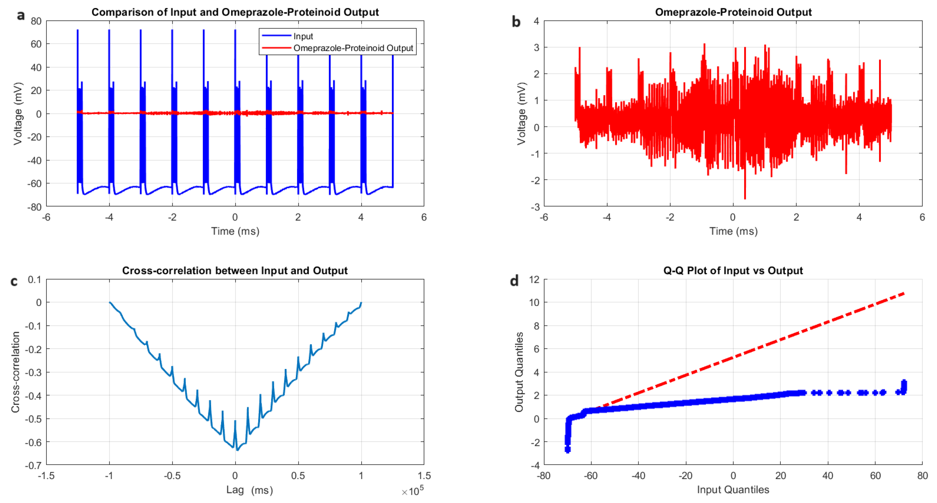
Figure 6.
Characterisation of induced-mode spiking in omeprazole–proteinoid samples. (a) Input–output comparison: Input signal (mean: mV, SD: 14.20 mV) and omeprazole–proteinoid output (mean: 0.34 mV, SD: 0.40 mV). Correlation coefficient: 0.6644, RMSE: 62.8671 mV. (b) Detailed output plot showing the response characteristics of the omeprazole–proteinoid sample (range: mV to 3.14 mV). (c) Cross-correlation analysis revealing a time lag of 1590 ms between input and output signals. Maximum difference: 71.91 mV at 2.00 ms. (d) Q-Q plot comparing the input and output distributions (Kolmogorov–Smirnov test: KS statistic = 0.9844, p < 0.0001), indicating significantly different signal distributions. The blue dots represent the actual data points, while the red dashed line represents the theoretical line for a normal distribution.
Figure 7.
Characterisation of phasic spiking dynamics in omeprazole–proteinoid complexes. (a) Input–output comparison: Input signal (mean: mV, SD: 8.23 mV) and omeprazole–proteinoid output (mean: 0.54 mV, SD: 0.33 mV). Correlation coefficient: 0.4503, RMSE: 55.9366 mV. (b) Detailed output plot illustrating the response characteristics of the omeprazole–proteinoid complex (range: mV to 3.17 mV). (c) Cross-correlation analysis revealing a time lag of ms between input and output signals. Maximum difference: 67.00 mV at 2.00 ms. (d) Q-Q plot comparing input and output distributions (Kolmogorov–Smirnov test: KS statistic = 0.9945, p < 0.0001), demonstrating significantly different signal distributions and non-linear response properties.
Figure 8.
Characterisation of tonic spiking dynamics in the omeprazole–proteinoid complexes. (a) Input–output comparison: Input signal (mean: mV, SD: 20.55 mV) and omeprazole–proteinoid output (mean: 0.80 mV, SD: 0.48 mV). Correlation coefficient: 0.6823, RMSE: 43.2821 mV. (b) Detailed output plot illustrating the sustained response characteristics of the omeprazole–proteinoid complex (range: mV to 3.63 mV). (c) Cross-correlation analysis revealing a time lag of -1231 samples between input and output signals. Maximum difference: 62.11 mV at 0.56 ms. (d) Q-Q plot comparing input and output distributions (Kolmogorov–Smirnov test: KS statistic = 0.9276, p < 0.0001), demonstrating significantly different signal distributions and non-linear response properties in tonic spiking mode. The blue dots are the data points. The red dashed line is the theoretical normal distribution.
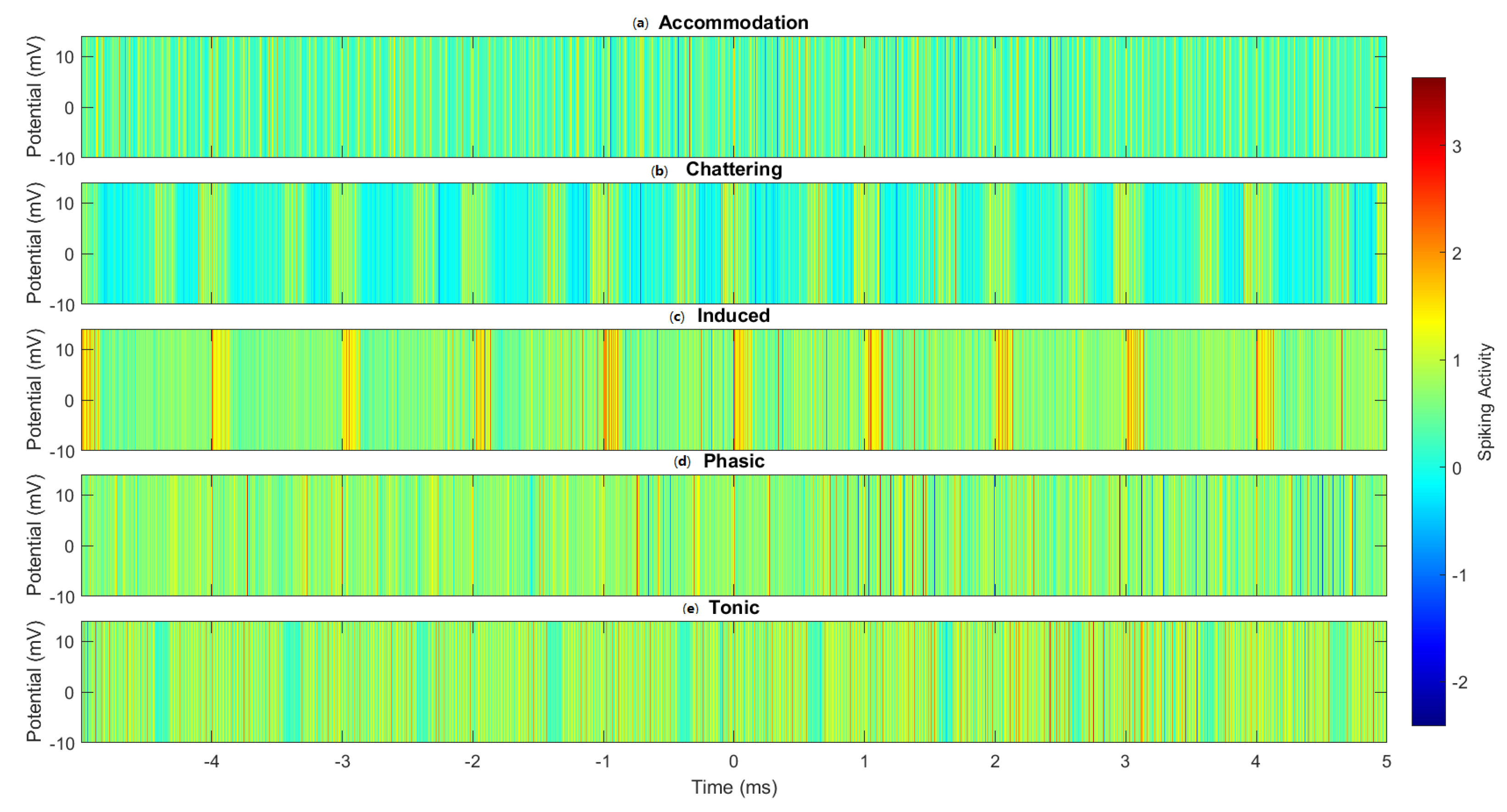
Figure 9.
Heatmap visualisation of the spike patterns across different spiking modes in omeprazole–proteinoid complexes. (a) Accommodation, (b) Chattering, (c) Induced, (d) Phasic, and (e) Tonic spiking modes. Colour intensity represents the membrane potential, with warmer colours indicating higher potentials. The heatmap reveals distinct temporal patterns and intensity distributions characteristic of each spiking mode, highlighting the complex- and mode-specific signal processing capabilities of the omeprazole–proteinoid system.
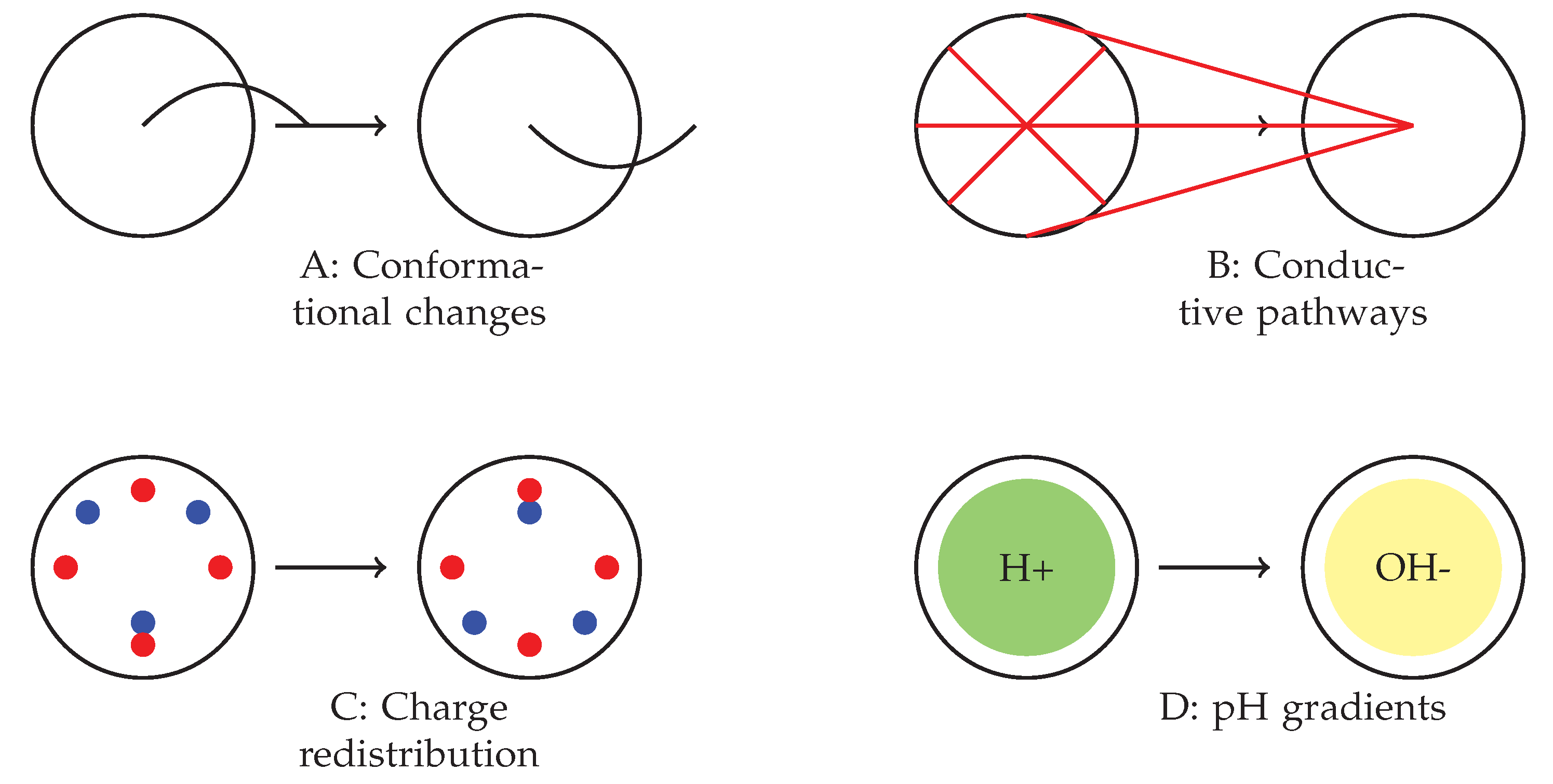
Figure 10.
Proposed mechanisms underlying the observed spiking behaviour in omeprazole–proteinoid complexes. (A) Voltage-sensitive conformational changes in the proteinoid structure. (B) Formation and breakdown of temporary conductive pathways. (C) Charge accumulation and redistribution processes. (D) Interactions between omeprazole’s proton pump inhibition and local pH gradients. The interplay between these mechanisms likely contributes to the complex, mode-dependent signal processing observed across different spiking regimes.
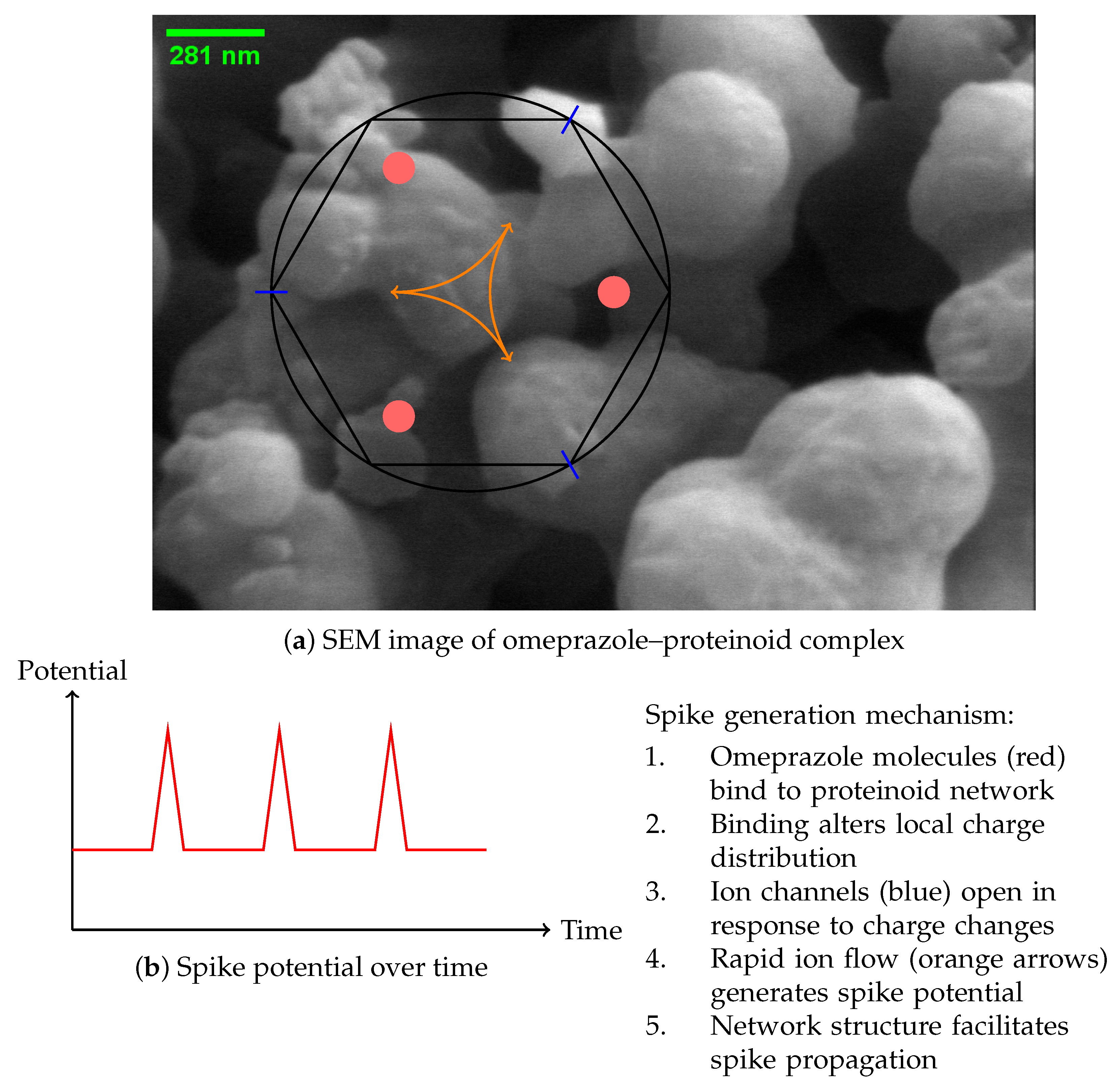
Figure 11.
Proposed mechanism for the generation of spikes in complexes formed by proteinoids and omeprazole. (a) SEM image showing the complex network structure. Schematic representation of the spike generation mechanism, illustrating omeprazole binding sites (red), ion channels (blue), and charge movement (orange arrows). (b) Graph illustrating the temporal evolution of the spike potential.
Table 1.
Comparison of proton pump inhibitors.
Table 1.
Comparison of proton pump inhibitors.
| PPI | Chemical Formula | Half-Life (h) | pKa | Reference |
|---|
| Omeprazole | C17H19N3O3S | 1.0 | 4.0 | [10] |
| Esomeprazole | C17H19N3O3S | 1.5 | 4.0 | [23,27] |
| Lansoprazole | C16H14F3N3O2S | 1.5 | 4.0 | [24] |
| Pantoprazole | C16H15F2N3O4S | 1.0 | 3.9 | [25] |
| Rabeprazole | C18H21N3O3S | 1.0 | 4.9 | [26] |
Table 2.
Summary of Izhikevich neuron input and omeprazole–proteinoid output characteristics for accommodation spiking model. This table presents the key metrics comparing the input signal generated by the Izhikevich neuron model configured for accommodation spiking and the corresponding output from the omeprazole–proteinoid complex. Accommodation spiking is characterised by a gradual increase in interspike intervals in response to sustained stimulation. The significant differences in mean, standard deviation, and range between the input and output highlight the complex signal processing occurring within the omeprazole–proteinoid system. Comparative metrics, including correlation coefficient and time lag, provide insights into the temporal relationship between input and output signals. The Kolmogorov–Smirnov test results confirm the statistically significant difference in signal distributions, underscoring the non-linear transformation induced by the omeprazole–proteinoid complex on the accommodation spiking pattern.
| Metric | Input Signal | Omeprazole–Proteinoid Output |
|---|
| Mean (mV) | | 0.60 |
| Standard deviation (mV) | 15.30 | 0.43 |
| Maximum (mV) | 72.50 | 3.99 |
| Minimum (mV) | | |
| Comparative Metrics |
| Correlation coefficient | 0.6841 |
| Root mean square error (mV) | 50.4592 |
| Maximum difference (mV) | 71.92 at 1.39 ms |
| Time lag (ms) | |
| Kolmogorov–Smirnov test |
| H-value | 1 (distributions are different) |
| p-value | <0.0001 |
| KS statistic | 0.9709 |
Table 3.
Comparative analysis of input signal and omeprazole–proteinoid output characteristics under chattering spiking stimulation. The table displays important statistical parameters for the omeprazole–proteinoid sample’s input signal and output response. The results showed that the correlation coefficient between the input and output was 0.79, the time lag was ms, the greatest variance was 75.71 mV (at time ms), and the root mean square error (RMSE) was 59.3 mV. A Kolmogorov–Smirnov test revealed that the input and output signals had significantly different distributions (KS statistic = 0.9717, p < 0.0001). These findings show that the omeprazole–proteinoid sample significantly changed the signal while retaining a moderate correlation with the input patterns.
| Metric | Input Signal | Omeprazole–Proteinoid Output |
|---|
| Mean (mV) | | 0.48 |
| Standard deviation (mV) | 19.72 | 0.51 |
| Maximum (mV) | 72.50 | 4.24 |
| Minimum (mV) | | |
Table 4.
Summary of Izhikevich neuron input and omeprazole–proteinoid output characteristics for induced spiking mode. This table presents a comparison between the input signal generated by the Izhikevich neuron model configured for induced spiking and the corresponding output from the omeprazole–proteinoid complex. The input signal’s wide voltage range ( mV to 72.21 mV) is dramatically compressed in the output ( mV to 3.14 mV), indicating a powerful attenuation effect. The positive mean of the output (0.34 mV) compared to the negative input mean ( mV) suggests a baseline shift in the signal processing. The moderate correlation coefficient (0.6644) implies that, while the output preserves some characteristics of the input, substantial non-linear processing occurs. The large time lag of 1590 ms points to complex internal dynamics within the omeprazole–proteinoid complex, possibly involving slow chemical or conformational changes. The high RMSE (62.8671 mV) and maximum difference (71.91 mV) further quantify the extent of signal transformation. The Kolmogorov–Smirnov test results (KS statistic = 0.9844, p < 0.0001) confirm that the input and output signals follow significantly different distributions, underscoring the non-linear nature of the signal processing in the omeprazole–proteinoid system during induced spiking stimulation.
| Metric | Input Signal | Omeprazole–Proteinoid Output |
|---|
| Mean (mV) | | 0.34 |
| Standard deviation (mV) | 14.20 | 0.40 |
| Maximum (mV) | 72.21 | 3.14 |
| Minimum (mV) | | |
| Comparative Metrics |
| Correlation coefficient | 0.6644 |
| Root mean square error (mV) | 62.8671 |
| Maximum difference (mV) | 71.91 at 2.00 ms |
| Time lag (ms) | 1590 |
| Kolmogorov–Smirnov Test |
| H-value | 1 (distributions are different) |
| p-value | <0.0001 |
| KS statistic | 0.9844 |
Table 5.
Summary of phasic spiking characteristics in omeprazole–proteinoid complexes. This table presents a detailed comparison between the input signal from the Izhikevich neuron model configured for phasic spiking and the output from the omeprazole–proteinoid complex. The results reveal significant signal transformation by the omeprazole–proteinoid system. The input signal’s wide voltage range ( mV to 62.46 mV) is markedly compressed in the output ( mV to 3.17 mV), demonstrating strong attenuation. The shift from a negative input mean ( mV) to a positive output mean (0.54 mV) suggests a fundamental change in signal characteristics. The reduced standard deviation in the output (0.33 mV vs. 8.23 mV input) indicates a smoothing effect. The low correlation coefficient (0.4503) implies substantial non-linear processing, more pronounced than in other spiking modes. The negative time lag of ms is particularly noteworthy, suggesting anticipatory behaviour in the omeprazole–proteinoid complex. This contrasts with the positive lag observed in induced spiking, highlighting mode-specific processing. The high RMSE (55.9366 mV) and maximum difference (67.00 mV) further quantify the extent of signal transformation. The Kolmogorov–Smirnov test results (KS statistic = 0.9945, p < 0.0001) indicate the most significant distributional difference among all spiking modes studied, emphasising the unique processing characteristics of the omeprazole–proteinoid system during phasic spiking stimulation.
| Metric | Input Signal | Omeprazole–Proteinoid Output |
|---|
| Mean (mV) | | 0.54 |
| Standard deviation (mV) | 8.23 | 0.33 |
| Maximum (mV) | 62.46 | 3.17 |
| Minimum (mV) | | |
| Comparative Metrics |
| Correlation coefficient | 0.4503 |
| Root mean square error (mV) | 55.9366 |
| Maximum difference (mV) | 67.00 at 2.00 ms |
| Time Lag (ms) | |
| Kolmogorov–Smirnov Test |
| H-value | 1 (distributions are different) |
| p-value | <0.0001 |
| KS statistic | 0.9945 |
Table 6.
Summary of tonic spiking characteristics in omeprazole–proteinoid complexes. This table presents an analysis of the input signal from the Izhikevich neuron model configured for tonic spiking and the corresponding output from the omeprazole–proteinoid complex. The results reveal significant and unique signal processing by the omeprazole–proteinoid system under tonic stimulation. The input signal’s broad voltage range ( mV to 62.17 mV) is substantially compressed in the output ( mV to 3.63 mV), demonstrating potent signal attenuation. Notably, the mean potential shifts from a negative input ( mV) to a positive output (0.80 mV), the highest positive shift observed among all spiking modes, suggesting a robust baseline alteration in signal characteristics. The dramatic reduction in standard deviation (from 20.55 mV to 0.48 mV) indicates a strong smoothing effect, potentially filtering out the high-frequency components of the input signal. The correlation coefficient (0.6823) is higher than in phasic mode but comparable to induced mode, implying a more linear relationship between the input and output while still preserving significant non-linear processing. The negative time lag of ms is the largest among all modes, suggesting a highly pronounced anticipatory behaviour in the omeprazole–proteinoid complex under tonic stimulation. This could indicate the development of a strong predictive response mechanism during sustained, regular input. The root mean square error (43.2821 mV) is the lowest among all modes, suggesting that tonic spiking may induce the most consistent and predictable response in the complex. The Kolmogorov–Smirnov test results (KS statistic = 0.9276, p < 0.0001), while still indicating significantly different distributions, show the lowest KS statistic among all modes. This suggests that the output distribution in tonic mode, while distinct, may be closer to the input distribution compared to other spiking patterns.
| Metric | Input Signal | Omeprazole–Proteinoid Output |
|---|
| Mean (mV) | | 0.80 |
| Standard deviation (mV) | 20.55 | 0.48 |
| Maximum (mV) | 62.17 | 3.63 |
| Minimum (mV) | | |
| Comparative Metrics |
| Correlation coefficient | 0.6823 |
| Root mean square error (mV) | 43.2821 |
| Maximum difference (mV) | 62.11 at 0.56 ms |
| Time lag (ms) | |
| Kolmogorov–Smirnov Test |
| H-value | 1 (distributions are different) |
| p-value | <0.0001 |
| KS statistic | 0.9276 |


