Machine-Learning-Based Prediction of Plant Cuticle–Air Partition Coefficients for Organic Pollutants: Revealing Mechanisms from a Molecular Structure Perspective

Abstract

Accurately predicting plant cuticle–air partition coefficients (K_ca) is essential for assessing the ecological risk of organic pollutants and elucidating their partitioning mechanisms. The current work collected 255 measured K_ca values from 25 plant species and 106 compounds (dataset (I)) and averaged them to establish a dataset (dataset (II)) containing K_ca values for 106 compounds. Machine-learning algorithms (multiple linear regression (MLR), multi-layer perceptron (MLP), k-nearest neighbors (KNN), and gradient-boosting decision tree (GBDT)) were applied to develop eight QSPR models for predicting K_ca. The results showed that the developed models had a high goodness of fit, as well as good robustness and predictive performance. The GBDT-2 model ($R_{\mathrm{adj}}^2$ = 0.925, $Q_{\mathrm{LOO}}^2$ = 0.756, $Q_{\mathrm{BOOT}}^2$ = 0.864, $R_{\mathrm{ext}}^2$ = 0.837, $Q_{\mathrm{ext}}^2$ = 0.811, and CCC = 0.891) is recommended as the best model for predicting K_ca due to its superior performance. Moreover, interpreting the GBDT-1 and GBDT-2 models based on the Shapley additive explanations (SHAP) method elucidated how molecular properties, such as molecular size, polarizability, and molecular complexity, affected the capacity of plant cuticles to adsorb organic pollutants in the air. The satisfactory performance of the developed models suggests that they have the potential for extensive applications in guiding the environmental fate of organic pollutants and promoting the progress of eco-friendly and sustainable chemical engineering.

1. Introduction

Natural and human activities release massive quantities of organic pollutants into the atmosphere [1]. These pollutants are intercepted by terrestrial vegetation and transferred to terrestrial ecosystems, where they accumulate through the food chain to higher nutrient levels [2,3]. The plant cuticle acts as the main interface for the exchange of organic pollutants between the air phase and the plant. It also serves as the main barrier to the interception of atmospheric pollutants [4]. Apart from the uptake and release of organic pollutants, the plant cuticle is also recognized as an accumulation chamber for organic pollutants [5,6]. The partitioning of organic compounds between the cuticle and air is of great interest due to airborne organic pollutants’ strong affinity to plant cuticles and their potential toxicity [7].

The exchange of organic contaminants between plant cuticles and air is typically evaluated through the plant cuticle–air partition coefficient (K_ca) [8,9]. The partition coefficient, K_ca, is generally determined by the ratio of the equilibrium concentration of organic contaminants between the isolated cuticle membranes (CMs) or polymer matrix membranes (MX) and the air, indicating the plant’s capacity to uptake airborne organic pollutants [10,11]. It is important to note that, at present, there is a paucity of experimentally measured K_ca values, and the interaction mechanisms of organic pollutants between plant cuticles and air are still obscure [12]. To the best of our knowledge, only a few hundred K_ca values for organic pollutants between a few plants and air have been measured experimentally [6]. The scarcity of these experimental K_ca values is mainly attributed to the laborious and time-consuming nature of conducting experiments to measure them, as well as the challenges posed by the diversity of plant species and types of organic contaminants [13,14]. This has also become an insurmountable bottleneck in assessing the ecological risk of organic pollutants by understanding their accumulation in plants and the exchange between the atmosphere and plants. Therefore, it could be valuable to focus on a straightforward and efficient method for predicting the K_ca values of organic pollutants to assess air quality and associated ecological risks.

Developing models with the ability to capture the molecular interactions between different compounds and plant cuticles is a complex task. When few independent variables are included, it is difficult, or sometimes even impossible, for a model to adequately reflect the mechanisms of interest precisely due to the limited number of independent variables available, which are representative of the influencing factors [2,15]. Some studies have solved this problem by developing poly-parameter linear free-energy relationship (pp-LFER) models [6,10]. However, the application of these models has been limited by the scarcity of Abrahamic descriptors and the fact that Abrahamic descriptors are not applicable to certain non-polar compounds [16]. This hinders the development and application of mechanism-based predictive models.

The relationship between the physical and chemical properties of the compound and the descriptors that quantify the molecular structural properties of compounds, namely the quantitative structural property relationship, provides a potential shortcut for clarifying the interaction between molecules and plant cuticles [17,18]. Currently, only one study has demonstrated the potential of QSPR models by developing a QSPR model for predicting K_ca [2]. However, the dataset used in this study contained only 49 log K_ca values, and these 49 organic compounds were measured with the same plant cuticle. The limited amount of available data poses a challenge to the development of a machine-learning model with a wide range of applications for assessing the ecotoxicity of compounds in various plant species.

Moreover, the challenge lies in capturing the complex relationship between K_ca and molecular structural properties from the increased amount of data and independent variables. Although the multiple linear regression (MLR) algorithm is convenient, efficient, and transparent in modeling, it is not applicable to complex nonlinear relationships, resulting in poor model performance [19]. We believe that the nonlinear machine-learning algorithm is the best candidate for K_ca prediction because of its powerful nonlinear processing capability [20,21]. For example, a study developed a QSPR model using the multi-layer perceptron (MLP) algorithm to predict the acute oral toxicity of pesticides in rats, achieving a high accuracy of 0.963 [22]. However, these types of models often have a “black box” nature [23]. Uncovering the dominant factors affecting the partitioning behavior of organic pollutants between plant cuticles and air from data and revealing their implicit effects while ensuring the predictability of the models is still a great challenge.

This study aimed to develop QSPR models by establishing relationships between measured K_ca values and molecular descriptors corresponding to organic pollutants in existing studies in order to ascertain the main mechanisms underlying the partitioning behavior of pollutants between the plant cuticle and the air. To achieve this, a comprehensive dataset of 255 K_ca values for 106 compounds and 25 plant species was collected to broaden the application domain of the models. In addition to the traditional linear algorithm (MLR), three popular nonlinear algorithms, namely MLP, k-nearest neighbors (KNN), and gradient-boosting decision tree (GBDT), were employed to develop QSPR models. Following the OECD guidelines [24], the models built using different machine-learning algorithms were rigorously and comprehensively evaluated to determine which of the QSPR models predicted K_ca most accurately. The application domains of the models were limited using the leverage method. Finally, the mechanism underlying plant cuticles’ adsorption of airborne organic pollutants was elucidated through the help of Shapley additive explanations (SHAP), thereby extracting some tacit or novel knowledge about the interaction between plant cuticles and organic pollutants. It is worth mentioning that the models developed in this study can estimate the accumulation of organics at the plant cuticle–air interface accurately even in the absence of experimental data, and they can provide valuable environmental information to guide the risk assessment and regulation of organic pollutants.

2. Results and Discussion

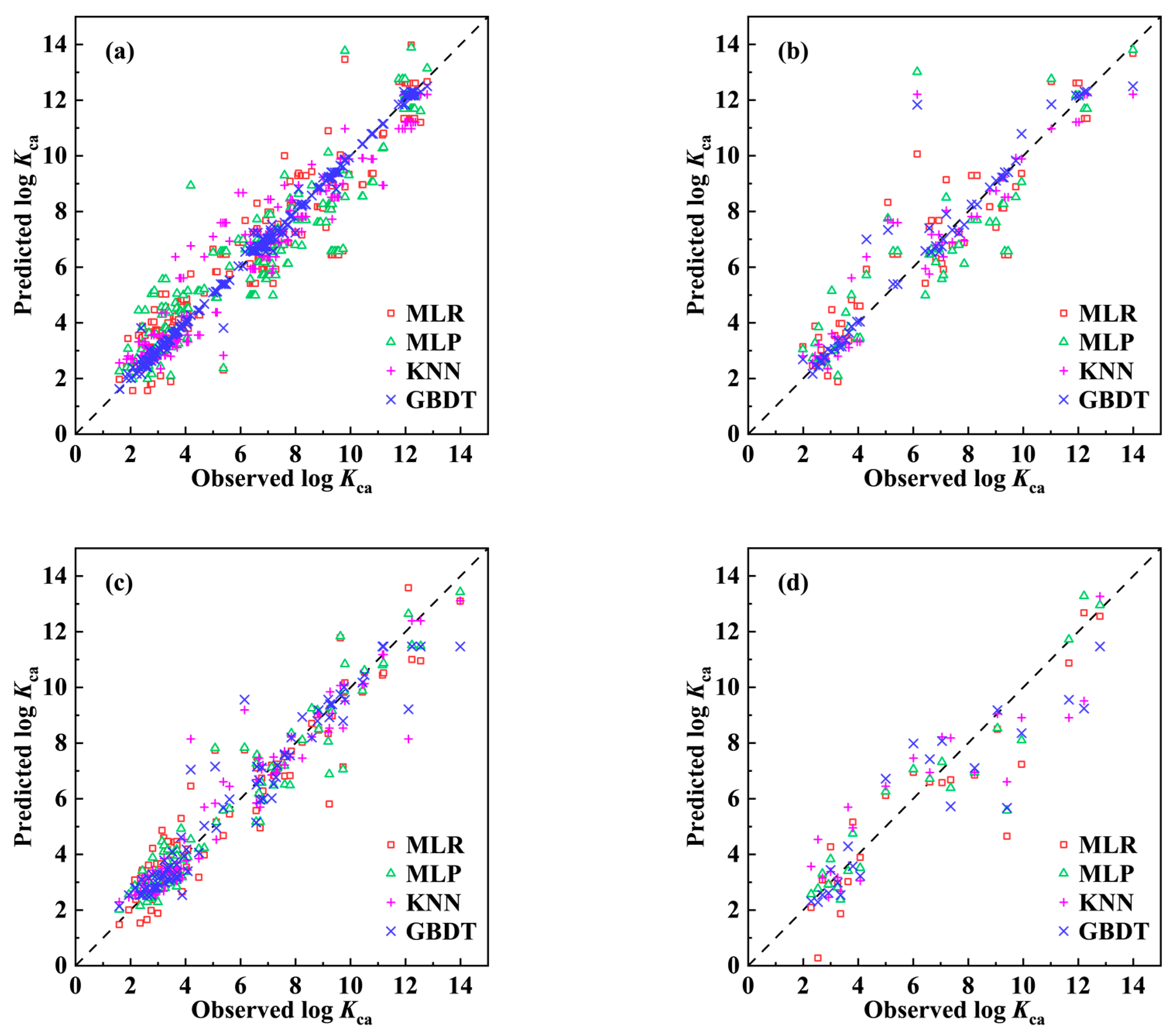
2.1. Development of the QSPR Model

The MLR algorithm selected the most appropriate descriptors from the pool of descriptors obtained from our initial screening and developed the QSPR models. Although the overall performance of the models improved as the number of descriptors increased (Figure S1), after the number of descriptors reached 5, descriptors with a VIF value greater than 10 were present in both datasets. Thus, the number of optimal descriptor combinations for both datasets was determined to be four after removing as much redundant information as possible for the QSPR models [25]. From Figure 1, it can be observed that the descriptors are not excessively correlated with each other. The selected best descriptors and their associated statistical indicators are presented in

Table 1. Descriptions involved in the final MLR models and corresponding statistical significance (p) and variance inflation factors (VIF) values.

Datasets	Descriptors	Parameters	p	VIF
(I)	VE1_L	coefficient sum of the last eigenvector (absolute values) from Laplace matrix	<0.001	7.527
	LLS_02	modified lead-like score from Monge et al. (8 rules)	<0.001	2.816
	H_Dz(p)	Harary-like index from Barysz matrix weighted by polarizability	<0.001	9.343
	SpMax2_Bh(v)	largest eigenvalue n. 2 of Burden matrix weighted by van der Waals volume	<0.001	2.937
(II)	SpPos_A	spectral positive sum from adjacency matrix	<0.001	6.594
	LLS_02	modified lead-like score from Monge et al. (8 rules)	<0.001	2.011
	LLS_01	modified lead-like score from Congreve et al. (6 rules)	<0.001	2.125
	SpMax2_Bh(v)	largest eigenvalue n. 2 of Burden matrix weighted by van der Waals volume	<0.001	3.128

Notes: Datasets (I): 255 experimental log K_ca values for 106 compounds; Datasets (II): average experimental log K_ca values for 106 compounds.

. The p-values of these eight descriptors are <0.5, indicating that they are statistically significant. The linear QSPR models developed with the selected descriptors were as follows:

MLR-1 (dataset (I)):

log K_ca = 2.006 VE1_L + 14.945 LLS_02 + 0.094 H_Dz(p) − 1.044 SpMax2_Bh(v) − 13.433

(1)

• n_tra = 204, $R_{\mathrm{adj}}^2$ = 0.873, $Q_{\mathrm{LOO}}^2$ = 0.869, $Q_{\mathrm{BOOT}}^2$ = 0.872, RMSE_tra = 1.101;
• n_ext = 51, $R_{\mathrm{ext}}^2$ = 0.839, $Q_{\mathrm{ext}}^2$ = 0.835, RMSE_ext = 1.296.

MLR-2 (dataset (II)):

log K_ca = 1.325 SpPos_A + 12.317 LLS_02 + 7.385 LLS_01 − 1.517 SpMax2_Bh(v) − 15.724

(2)

• n_tra = 84, $R_{\mathrm{adj}}^2$ = 0.891, $Q_{\mathrm{LOO}}^2$ = 0.874, $Q_{\mathrm{BOOT}}^2$ = 0.886, RMSE_tra = 0.987;
• n_ext = 22, $R_{\mathrm{ext}}^2$ = 0.833, $Q_{\mathrm{ext}}^2$ = 0.807, RMSE_ext = 1.466.

Three nonlinear algorithms, namely MLP, KNN, and GBDT, were employed to explore the nonlinear relationship between the K_ca of organic pollutants and their molecular structures, with a view to developing more accurate models. For the same dataset, the nonlinear models were trained using the same molecular descriptors as the linear models. Eventually, six nonlinear QSPR models were developed based on two datasets and three machine-learning algorithms. The results of the hyperparameter search for the models are presented in Table S1. The measured and predicted log K_ca values for the MLR-1 model, MLP-1 model, KNN-1 model, and GBDT-1 model are provided in Table S2, while the values associated with the models developed based on dataset (II) are presented in Table S3. The most stringent model validation criteria in the field of QSPR research were employed in this study to assess the performance of models, including $R_{\mathrm{adj}}^2$ > 0.7, $Q_{\mathrm{LOO}}^2$ > 0.6, $Q_{\mathrm{BOOT}}^2$ > 0.6, $R_{\mathrm{ext}}^2$ > 0.7, $Q_{\mathrm{ext}}^2$ > 0.6, CCC > 0.85, and minimize error values [26,27]. The values of the validation parameters for the eight QSPR models are shown in

Table 2. Statistical parameters in the training and test sets for models of K_ca.

Models	Training Set							Test Set
	ntra	${\mathit{R}}_{\mathbf{adj}}^2$	${\mathit{Q}}_{\mathbf{LOO}}^2$	${\mathit{Q}}_{\mathbf{BOOT}}^2$	MAEtra	RMSEtra	stra	next	${\mathit{R}}_{\mathbf{ext}}^2$	${\mathit{Q}}_{\mathbf{ext}}^2$	MAEext	RMSEext	sext	CCC
Threshold	-	>0.7	>0.6	>0.6	-	-	-	-	>0.7	>0.6	-	-	-	>0.85
MLR-1	204	0.873	0.869	0.872	0.874	1.101	1.114	51	0.839	0.835	1.024	1.296	1.364	0.914
MLP-1		0.850	0.678	0.676	0.917	1.194	1.209		0.790	0.784	1.009	1.485	1.564	0.889
KNN-1		0.920	0.742	0.778	0.638	0.871	0.882		0.859	0.855	0.706	1.214	1.279	0.925
GBDT-1		0.995	0.936	0.964	0.114	0.224	0.227		0.911	0.902	0.411	1.001	1.054	0.952
MLR-2	84	0.891	0.874	0.886	0.725	0.987	1.018	22	0.833	0.807	1.006	1.466	1.668	0.902
MLP-2		0.921	0.798	0.809	0.629	0.843	0.869		0.887	0.884	0.798	1.139	1.296	0.940
KNN-2		0.919	0.661	0.802	0.536	0.855	0.881		0.821	0.815	1.176	1.435	1.632	0.891
GBDT-2		0.925	0.756	0.864	0.504	0.821	0.847		0.837	0.811	1.097	1.451	1.651	0.891

Notes: n_tra and n_ext: the number of chemicals in the training set and test set, respectively; $R_{\mathrm{adj}}^2$ and $R_{\mathrm{ext}}^2$: the correlation coefficient square between observed and fitted values in training set and test set, respectively; $Q_{\mathrm{LOO}}^2$: leave one out cross-validated Q²; $Q_{\mathrm{BOOT}}^2$: bootstrap method, 1/5, 5000 iterations; $Q_{\mathrm{ext}}^2$: external explained variance; s_tra: standard error of estimate for training set; s_ext: standard error of estimate for test set; CCC: concordance correlation coefficient.

.

As shown in Table 2, the $R_{\mathrm{adj}}^2$ (0.850–0.995) of the four models (MLR-1, MLP-1, KNN-1, and GBDT-1 model) developed based on dataset (I) exceeded the standard thresholds, demonstrating excellent goodness of fit. The stability parameters $Q_{\mathrm{LOO}}^2$ and $Q_{\mathrm{BOOT}}^2$ had values of 0.678–0.936 and 0.676–0.964, respectively, above the acceptable thresholds, indicating that the models are statistically robust and have fair internal accuracy [28]. In terms of external predictive power, the $R_{\mathrm{ext}}^2$ (0.790–0.911), $Q_{\mathrm{ext}}^2$ (0.784–0.902), and CCC (0.889–0.952) of these models were much greater than the strict standard thresholds, implying that all four models achieved fairly reasonable predictions [29]. The measured and predicted log K_ca values for the training and test sets are plotted in Figure 2a and Figure 2b, respectively. For the training and test sets of each model, the data points followed a similar discrete pattern, with all of them being close to the 1:1 line, proving that these four models had high-level accuracy and prediction abilities [30,31]. The consistency of the training and test set errors indicated that these models had similar internal and external prediction accuracies, confirming the excellent external prediction abilities of these models [30]. Overall, both the linear and nonlinear QSPR models developed based on dataset (I) were acceptable.

Multiple verification parameters were also calculated to evaluate the performance of the models (MLR-2, MLP-2, KNN-2, and GBDT-2 model) developed based on dataset (II) (Table 2). The internal validation results derived from the use of the data points in the training set were $R_{\mathrm{adj}}^2$ = 0.891–0.925, $Q_{\mathrm{LOO}}^2$ = 0.661–0.874, and $Q_{\mathrm{BOOT}}^2$ = 0.802–0.886, indicating that the models exhibited excellent internal predictability and stability. The external validation results derived from the use of the data points in the test set were $R_{\mathrm{ext}}^2$ = 0.821–0.887, $Q_{\mathrm{ext}}^2$ = 0.807–0.884, and CCC = 0.891–0.940, demonstrating the superior performance of the models in predicting external data. In addition, the error-based statistical metrics further demonstrated the “good” quality of these models in predicting log K_ca values for the training set and test set. Scatter plots of the log K_ca values measured and predicted by the four models developed using dataset (II) are shown in Figure 2c,d. The data points were more concentrated on the 1:1 line than those in dataset (I), indicating that the four models also have the appropriate ability to predict log K_ca values. The results of our rigorous validation testing indicated that these four models performed satisfactorily in various aspects.

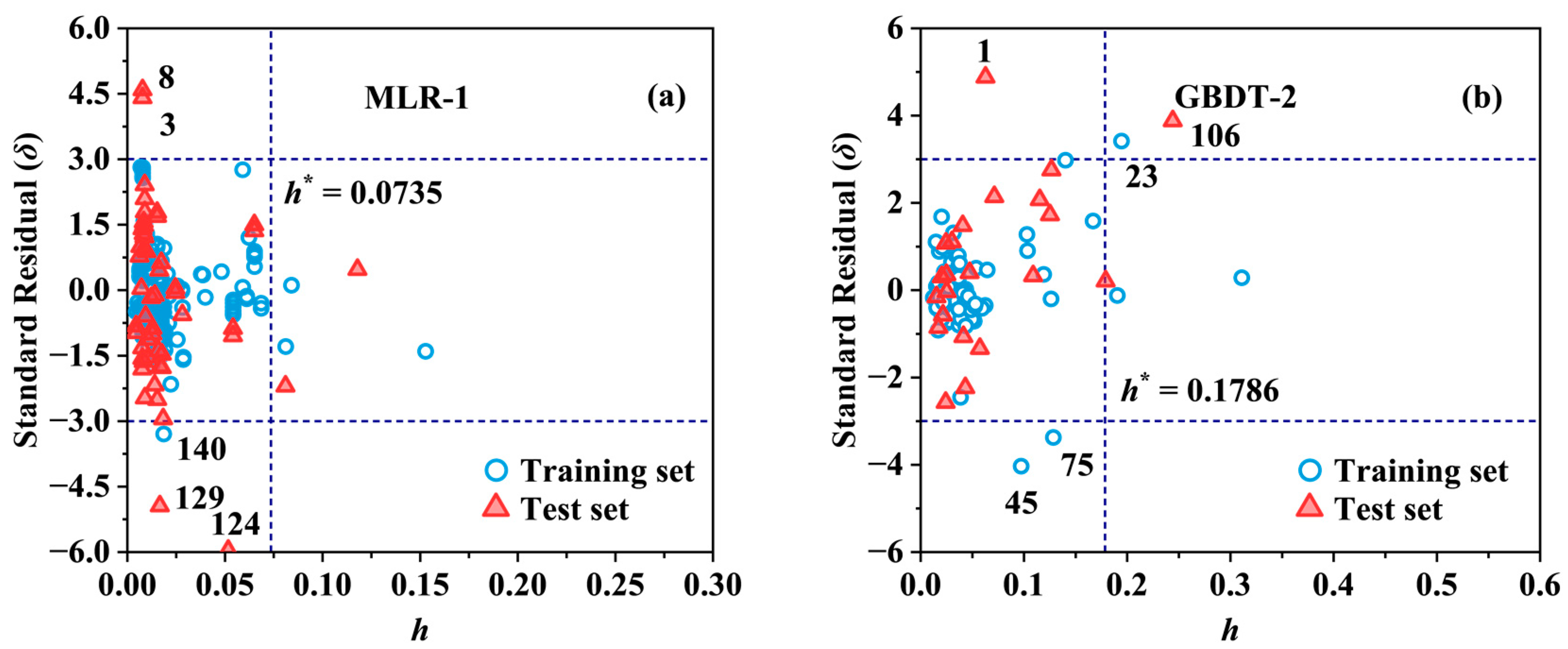
2.2. Applicability Domain

The Williams plots shown in Figure 3 and Figure S2 established the structure range of the compounds for which the model could reliably predict log K_ca values. Although structural outliers were found in all eight models, most of them fell into the category of “good high leverage” points with low δ (|δ| ≤ 3). These points were predicted with high accuracy, ensuring the stability and generalization performance of the models and extending their applicability domains to some extent [32,33]. The MLP-1, KNN-2, and GBDT-2 models contained one, two, and two structural outliers with |δ| > 3 as well (Figure S2a,f and Figure 3b), respectively. This may be caused by the unique structure of these three compounds and the limited structural representation of the selected descriptors [34]. Information related to the response outliers in datasets (I) and (II) is listed in Tables S4 and S5. Decachlorobiphenyl (ID: 124) and Tetrachlorobiphenyl (ID: 129) in dataset (I) were detected as response outliers in all of the four models developed by the four algorithms. This inaccurate prediction might have been caused by the fact that the molecular descriptors did not capture information about the key effects of plant cuticle adsorption on these two compounds [33]. In addition, the variability of the experimental values may also have an impact on the model predictions [35]. For example, the K_ca value for Hexachlorobenzene (ID: 74) was probably underestimated excessively by Gobas, McNeil, Lovett-Doust and Haffner [36], and, therefore, was not in the AD range of the KNN-1 model and the GBDT-1 model when compared to the value measured by Sabljic, Guesten, Schoenherr and Riederer [5] (log K_ca = 4.30 versus 6.78~7.28). By taking the mean value instead, the models developed based on dataset (II) predicted the K_ca value for Hexachlorobenzene (ID: 24) with good accuracy. Overall, the presence of most data points in the applicability domain demonstrated the validity and good performance of the models [37].

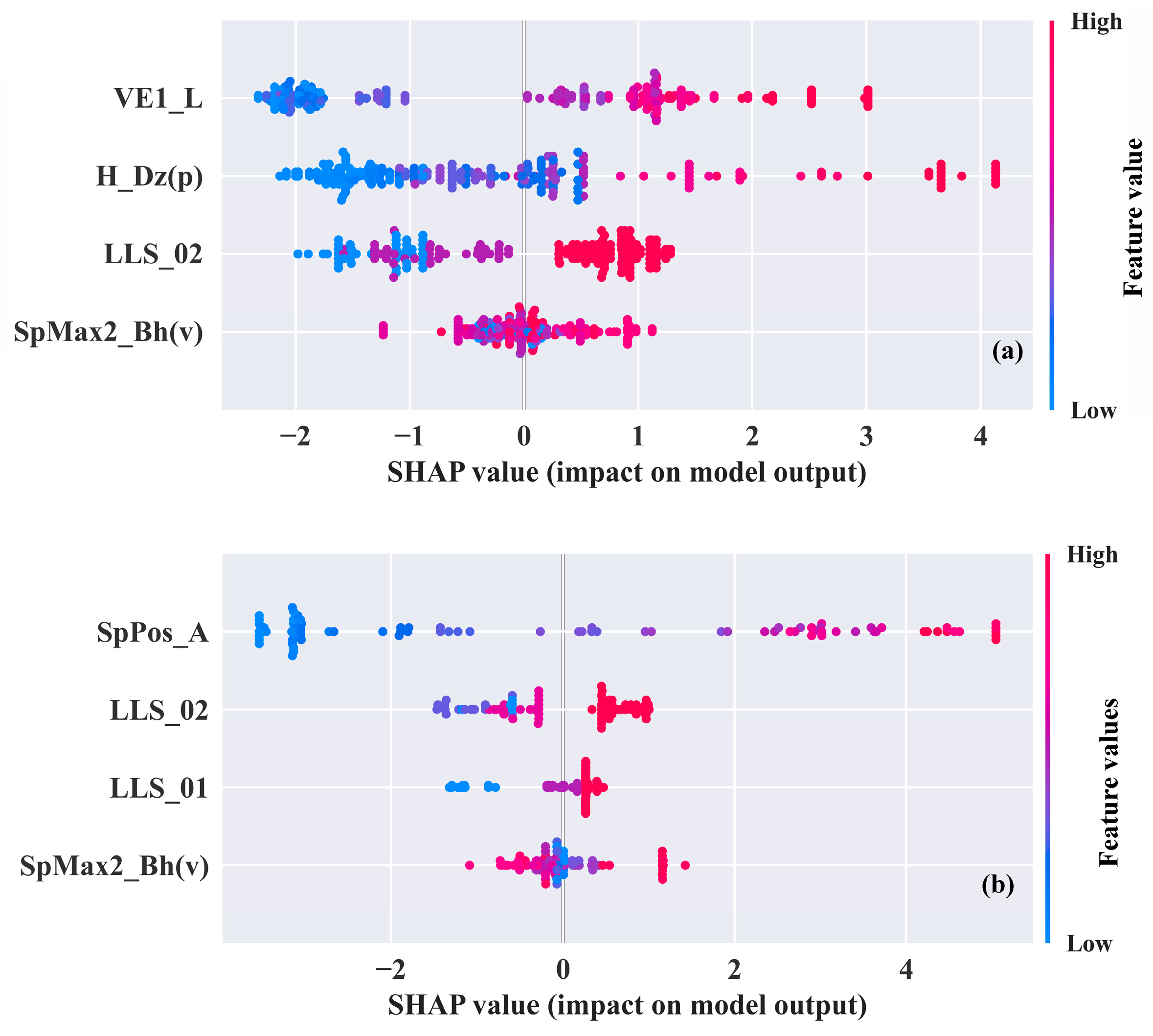
2.3. Mechanism Interpretation

In addition to assessing the performance of each model, SHAP values were analyzed to interpret both the GBDT-1 model and the GBDT-2 model and determine whether the models were consistent with known mechanisms [38]. The SHAP summary plot shown in Figure 4 succinctly and clearly shows the relationship between the SHAP values and each descriptor, making it easy to discern whether there is a positive or negative correlation between the descriptor and log K_ca. For example, compounds with a large VE1_L (red color) typically have higher SHAP values, indicating higher log K_ca values. Thus, the correlation between VE1_L and log K_ca can be considered positive. The descriptors are sorted on the y-axis in descending order by the mean of the absolute value of SHAP, i.e., the descriptor contribution.

Figure 4 shows that the contributions of LLS_02 and SpMax2_Bh(v) to log K_ca are consistently in the top four positions in both the GBDT-1 model and GBDT-2 model, suggesting that these two descriptors have a dominant effect on the plant cuticle’s capacity to adsorb organic pollutants. The descriptor LLS_02 is a lead-like score modified by Monge, Arrault, Marot and Morin-Allory [39], and it was used to screen compounds that qualify as leads in drug discovery [40]. The score was determined based on eight rules [39]: compounds that met all the rules had an LLS_02 value equal to 1, and the more rules that were violated, the lower the LLS_02 value [41]. From these eight rules, it was found that compounds with lower LLS_02 values had high molecular weights, as well as a high number of hydrogen bond donors and hydrogen bond acceptors. High-molecular-weight compounds are usually difficult to pass through phospholipid membranes, and increasing the number of hydrogen bond donors and hydrogen bond acceptors makes these compounds more hydrophilic [42]. Therefore, a decrease in log K_ca could be expected for compounds with lower LLS_02 values. The descriptor SpMax2_Bh(v) was largest eigenvalue n. 2 of Burden matrix weighted by van der Waals volume, and belonged to Burden eigenvalues [43]. Burden eigenvalues were calculated from the Burden matrix Bh(w), and the diagonal elements of the adjacency matrix are van der Waals volume. These values were related to molecular branching, the presence of heteroatoms, and bond multiplicity [44,45]. The van der Waals volume contributed to the lipophilicity of the molecule, and the increase in the SpMax2_Bh(v) value logically should have led to an increase in the K_ca value [46]. However, as presented in Figure 4a,b, how the SpMax2_Bh(v) values regulated the partitioning of organic pollutants between plant cuticles and the air was complicated. This might be due to the limited number of data points making it difficult for the models to adequately respond to the mechanisms involved. Similar to LLS_02, LLS_01 is a lead-like score. The score was determined by six rules (molecular weight, hydrogen bond donors, hydrogen bond acceptors, number of rotatable bonds, etc.) [47]. Therefore, there was also a positive correlation between LLS_01 and log K_ca.

The VE1_L, H_Dz(p), and SpPos_A belonged to the category of 2D matrix-based descriptors. The VE1_L was based on the Laplace matrix, which provides the number of spanning trees for molecular graphing. This quantity reflected the structural complexity of polycyclic molecules, with higher spanning-tree quantities indicating greater molecular structural complexity [48]. Generally, compounds with polycyclic structures were more stable and conducive to the adsorption of compounds by the plant cuticle, meaning that they should have shown increased K_ca values [29,49]. The descriptor H_Dz(p) was based on the Barysz matrix, weighted by the polarizability [50]. The Barysz matrix was considered to be related to the presence of heteroatoms and multiple bonds in molecules [48]. The magnitude of the polarizability was influenced by molecular size, structure, and electron distribution [51]. The greater the polarization rate, the stronger the polarity of the molecules, and the stronger the intermolecular interactions [52]. Molecules tended to distribute in the plant cuticle through intermolecular forces, leading to an increase in K_ca values [53]. The SpPos_A was calculated by summing the positive eigenvalues from the adjacency matrix, encoding information about molecular size, molecular branching, and molecular complexity [54,55,56]. Figure 4 indicates that log K_ca is proportional to SpPos_A.

According to the results of this study, molecular weight, molecular size, molecular branching, molecular complexity, the number of hydrogen bond donors, the number of hydrogen bond acceptors, the presence of heteroatoms, bond multiplicity, polycyclic structure, and polarizability are the main molecular structure features that affect the capacity of plant cuticles to adsorb airborne organic pollutants.

2.4. Model Comparison

To determine which model was most effective at predicting K_ca values, cumulative distribution plots of the residuals (Figure S3) were plotted to depict the predictive effectiveness of the eight models. As shown in Figure S3, if the residuals fall in the −1 to 1 interval with a higher percentage, the model predicts the log K_ca values more accurately. Our comparison among the four models developed based on dataset (I) indicated that the GBDT-1 model was significantly better than the other three models, while the GBDT-2 model was found to show the best performance among the four models developed based on dataset (II). The superiority of the GBDT-1 and GBDT-2 models in predicting the log K_ca values can also clearly be observed in the scatter plots of the real predicted values (Figure 2). Although the GBDT-1 model performed better than the GBDT-2 model in terms of the validation parameters (Table 2), the repetitive data points in dataset (I) exacerbated the risk of data leakage. Therefore, the GBDT-2 model is recommended as a useful tool for predicting the K_ca values of organic pollutants.

To further evaluate the eight QSPR models, several existing models for predicting log K_ca values were collected and compared. The differences in datasets, descriptors, and validation metrics between the different studies reporting these models increased the difficulty of the comparison. The details of the comparison are presented in Table S6. The number of compounds simulated in the early studies was not more than a hundred; the types of compounds were concentrated, and the distribution behavior was more regular, resulting in a high fitting accuracy for their models [2,10]. Eddula, Xu, Jiang, Huang, Tirumala, Liu, Acree and Abraham [6] collected 215 measured K_ca values and established pp-LFER models with excellent accuracy. However, the application of these models was limited by the number of descriptors. The existing studies applied only the MLR algorithm to develop models for predicting K_ca values and did not fully exploit any powerful nonlinear algorithms. In contrast, the QSPR models developed in this study showed excellent prediction accuracy while fitting more measured K_ca values. Further statistical analyses adequately demonstrated the reliability of these models. In addition, the nonlinear relationship between the plant cuticle–air partition coefficients and molecular descriptors of the compounds was established for the first time in this study.

3. Materials and Methods

3.1. Dataset Preparation

The data points for the experimental log K_ca dataset (dataset (I)), consisting of 255 data points measured for 106 compounds and 25 plant species, were collected from existing studies. Specifically, for compounds whose K_ca measured values had not been directly reported but their plant cuticle/water partition coefficient (K_cw) and gas/water partition coefficients (K_aw) had been reported, their log K_ca value was calculated as follows: log K_ca = log K_cw − log K_aw [10]. The plant species and tissue types used for the experimental measurements and the sources corresponding to each data point are listed in Table S7. The difference in the log K_ca values measured for each compound in different tissues of different plant species was very small, and the presence of these similar data points significantly increased the risk of data leakage. Therefore, the log K_ca values from different plant species and different tissue types were averaged in this study, resulting in dataset (II) containing the measured log K_ca values of 106 compounds (Table S8). The mean log K_ca values with standard deviation were 6.30 ± 3.14 for dataset (I) and 5.79 ± 3.15 for dataset (II). Following data quality testing (Figure 5), it was concluded that both dataset (I) and dataset (II) meet the Pauta criterion [57].

3.2. Descriptor Generation and Filtering

The molecular structure characterization information of the compounds was described through molecular descriptors [58]. After determining the molecular structures of the compounds, the geometric structures of the compounds were fully optimized using MM2 molecular mechanics [59]. A descriptor pool consisting of 5290 molecular descriptors was generated using alvaDesc software (Version 1.0.8) [60]. Preliminary descriptor screening was carried out in two steps, the first of which involved removing descriptors with missing, constant, and near-constant values, and the second of which involved identifying descriptors with pairwise correlations greater than 0.9 and removing one of the interrelated descriptors in order to reduce redundant information and make it easier to use the model in the future [61,62]. The remaining 165 and 163 descriptors of dataset (I) and dataset (II), respectively, were further filtered using the MLR algorithm in the next step. Detailed information about the steps of our further screening is presented below.

3.3. Model Development and Validation

The Y-ranking method was used to divide each dataset into a training set and a test set [63]. The training and test sets consisted of 80% and 20% log K_ca measured values and the corresponding molecular descriptors in the dataset, respectively [64,65]. The training sets were used to develop and internally validate each model, whereas the test set was solely dedicated to validating each model’s performance in predicting the K_ca for new compounds [66]. One linear algorithm (MLR) and three common nonlinear algorithms—MLP, KNN, and GBDT—were used to develop models for both datasets, resulting in 8 QSPR models. These 8 models were named in the format of “modeling algorithm + dataset number”. For example, the QSPR model developed using the KNN algorithm based on dataset (I) was named the KNN-1 model. Further details on these four machine-learning algorithms are provided in Text S1.

Identifying and selecting descriptors that contribute significantly to the dependent variable is essential for QSPR modeling. In this study, further screening of the descriptors was carried out using stepwise MLR in SPSS (Version 20.0) software [67]. Generally, the model developed using the best descriptor combination should have a high $R_{\mathrm{adj}}^2$ and $Q_{\mathrm{ext}}^2$ and the lowest possible number of descriptors [68]. Additionally, multicollinearity between descriptors was assessed using the variance inflation factor (VIF). The VIF of each descriptor should be less than 10 to avoid excessive inter-correlation between descriptors [69]. The MLR-1 and MLR-2 models were developed by establishing the relationship between measured log K_ca values and the best descriptor combinations based on dataset (I) and dataset (II), respectively.

The machine-learning library scikit-learn in Python (Version 3.9.6) was utilized to train the nonlinear QSPR models developed by the other three machine-learning algorithms [70]. With the help of the GridSearchCV function in the sklearn library, a grid search and five-fold cross-validation were performed to optimize various hyperparameters of models [71]. Table S1 lists these hyperparameters and their ranges for each model, as well as the modules for the different machine-learning algorithm implementations. Each modeling process of different ML algorithms took the best combination of descriptors screened by MLR as the independent variable to ensure consistency in the comparison among the models.

In accordance with the fourth principle of the OECD guidelines, assessing the fit, stability, and predictive performance of QSPR models with a wide range of internally and externally validated statistical parameters was essential for understanding the predictive quality of new compounds and ensuring the reliability of the developed models [72]. $R_{\mathrm{adj}}^2$, MAE_tra, RMSE_tra, and s_tra were used to measure the goodness of fit of the models [73,74]. Internal robustness was characterized by performing leave-one-out cross-validation and bootstrap cross-validation based on $Q_{\mathrm{LOO}}^2$ and $Q_{\mathrm{BOOT}}^2$ [75,76,77]. Each model’s external predictive ability was assessed based on $R_{\mathrm{ext}}^2$, $Q_{\mathrm{ext}}^2$, CCC, and three error-based metrics [78,79]. The leverage value method was employed to limit the compound structure space in which the model could reliably predict log K_ca [28]. In addition, Williams plots of leverage values (h_i) versus normalized residuals (δ) were applied to visualize the applicability domains of the QSPR models. In addition, response outliers (the point with |δ| > 3) and structural outliers (the point with h > h*) could be clearly identified from the plots [80,81]. The formulas for h_i, h*, and δ are presented in Text S3.

3.4. Model Interpretation

Understanding how dominant features affect model predictions is another important principle in QSPR model development [24]. The SHAP method was applied to explain the models developed using the GBDT algorithm and determine the effect of specific structural features of molecules on plant cuticles’ adsorption of airborne organic pollutants [82]. The SHAP value of a feature is determined by the average of the feature’s contribution across all possible feature alignments in the feature set [38]. It measures the degree and direction of the descriptor’s contribution to the prediction result: higher absolute SHAP values indicate a higher contribution, and whether a SHAP value demonstrates positivity or negativity corresponds to the positive and negative impact of the descriptor on the prediction result [83,84]. The global importance of a feature is reflected by averaging the absolute SHAP values corresponding to all the samples in that feature [85]. The formula for calculating SHAP values and more information about them are presented in Text S4.

4. Conclusions

K_ca is a key factor in assessing the capacity of plant cuticles to adsorb airborne organic pollutants. However, the development of reliable predictive tools to estimate K_ca has been hampered by the complexity of the molecular structures of organic pollutants. In this study, we established a comprehensive K_ca dataset that covers 255 experimental log K_ca values for 106 compounds in 25 plant species and 3 tissue types (dataset (I)). Additionally, 255 data points were averaged to form a second dataset (dataset (II)) containing 106 measured log K_ca values for 106 compounds. Based on these two datasets, eight QSPR models designed to predict K_ca values were developed using four machine-learning algorithms (MLR, MLP, KNN, and GBDT). Rigorous validation testing indicated that these models have acceptable fit, stability, and external predictive power. In addition, the GBDT-1 model ($R_{adj}^2$ = 0.995, $Q_{LOO}^2$ = 0.936, $Q_{BOOT}^2$ = 0.964, $R_{ext}^2$ = 0.911, $Q_{ext}^2$ = 0.902, and CCC = 0.952) and the GBDT-2 model ($R_{adj}^2$ = 0.925, $Q_{LOO}^2$ = 0.756, $Q_{BOOT}^2$ = 0.864, $R_{ext}^2$ = 0.837, $Q_{ext}^2$ = 0.811, and CCC = 0.891) showed the best performance on datasets (I) and (II), respectively. The GBDT-2 model can be recommended as the best tool for predicting K_ca values due to its low risk of data leakage. Interpreting the GBDT-1 and GBDT-2 models using the SHAP method revealed that molecular weight, molecular complexity, the number of hydrogen bond donors, the number of hydrogen bond acceptors, and polarizability are the most important factors that affect K_ca predictions. In summary, the models presented in this work provided a fast and reliable method for obtaining K_ca values, overcoming the obstacles of experimental challenges, halting kinetic models, and mistake-prone theoretical calculations. We hope that our findings will inspire the refinement of the modeling process to help with predicting other physicochemical properties using comparable workflows.

References

1. Talaiekhozani, A.; Rezania, S.; Kim, K.-H.; Sanaye, R.; Amani, A.M. Recent advances in photocatalytic removal of organic and inorganic pollutants in air. J. Clean. Prod. 2021, 278, 123895. [Google Scholar] [CrossRef]
2. Welke, B.; Ettlinger, K.; Riederer, M. Sorption of Volatile Organic Chemicals in Plant Surfaces. Environ. Sci. Technol. 1998, 32, 1099–1104. [Google Scholar] [CrossRef]
3. Li, Q.; Chen, B. Organic Pollutant Clustered in the Plant Cuticular Membranes: Visualizing the Distribution of Phenanthrene in Leaf Cuticle Using Two-Photon Confocal Scanning Laser Microscopy. Environ. Sci. Technol. 2014, 48, 4774–4781. [Google Scholar] [CrossRef]
4. Collins, C.D.; Finnegan, E. Modeling the Plant Uptake of Organic Chemicals, Including the Soil−Air−Plant Pathway. Environ. Sci. Technol. 2010, 44, 998–1003. [Google Scholar] [CrossRef] [PubMed]
5. Sabljic, A.; Guesten, H.; Schoenherr, J.; Riederer, M. Modeling plant uptake of airborne organic chemicals. 1. Plant cuticle/water partitioning and molecular connectivity. Environ. Sci. Technol. 1990, 24, 1321–1326. [Google Scholar] [CrossRef]
6. Eddula, S.; Xu, A.; Jiang, C.; Huang, J.; Tirumala, P.; Liu, G.; Acree, W.E.; Abraham, M.H. Abraham solvation parameter model: Updated correlations for describing solute partitioning into plant cuticles from water and from air. Phys. Chem. Liq. 2021, 59, 716–732. [Google Scholar] [CrossRef]
7. Chefetz, B.; Xing, B. Relative Role of Aliphatic and Aromatic Moieties as Sorption Domains for Organic Compounds: A Review. Environ. Sci. Technol. 2009, 43, 1680–1688. [Google Scholar] [CrossRef]
8. Wang, Y.; Zhang, Z.; Tan, F.; Rodgers, T.F.M.; Hou, M.; Yang, Y.; Li, X. Ornamental houseplants as potential biosamplers for indoor pollution of organophosphorus flame retardants. Sci. Total Environ. 2021, 767, 144433. [Google Scholar] [CrossRef]
9. Zhao, X.; He, M.; Shang, H.; Yu, H.; Wang, H.; Li, H.; Piao, J.; Quinto, M.; Li, D. Biomonitoring polycyclic aromatic hydrocarbons by Salix matsudana leaves: A comparison with the relevant air content and evaluation of environmental parameter effects. Atmos. Environ. 2018, 181, 47–53. [Google Scholar] [CrossRef]
10. Platts, J.A.; Abraham, M.H. Partition of Volatile Organic Compounds from Air and from Water into Plant Cuticular Matrix:  An LFER Analysis. Environ. Sci. Technol. 2000, 34, 318–323. [Google Scholar] [CrossRef]
11. Keymeulen, R.; De Bruyn, G.; Van Langenhove, H. Headspace gas chromatographic determination of the plant cuticle–air partition coefficients for monocyclic aromatic hydrocarbons as environmental compartment. J. Chromatogr. 1997, 774, 213–221. [Google Scholar] [CrossRef]
12. Barber, J.L.; Thomas, G.O.; Kerstiens, G.; Jones, K.C. Current issues and uncertainties in the measurement and modelling of air–vegetation exchange and within-plant processing of POPs. Environ. Pollut. 2004, 128, 99–138. [Google Scholar] [CrossRef] [PubMed]
13. Huang, S.; Dai, C.; Zhou, Y.; Peng, H.; Yi, K.; Qin, P.; Luo, S.; Zhang, X. Comparisons of three plant species in accumulating polycyclic aromatic hydrocarbons (PAHs) from the atmosphere: A review. Environ. Sci. Pollut. Res. 2018, 25, 16548–16566. [Google Scholar] [CrossRef] [PubMed]
14. Fernández, V.; Bahamonde, H.A.; Javier Peguero-Pina, J.; Gil-Pelegrín, E.; Sancho-Knapik, D.; Gil, L.; Goldbach, H.E.; Eichert, T. Physico-chemical properties of plant cuticles and their functional and ecological significance. J. Exp. Bot. 2017, 68, 5293–5306. [Google Scholar] [CrossRef]
15. Qi, X.; Li, X.; Yao, H.; Huang, Y.; Cai, X.; Chen, J.; Zhu, H. Predicting plant cuticle-water partition coefficients for organic pollutants using pp-LFER model. Sci. Total Environ. 2020, 725, 138455. [Google Scholar] [CrossRef] [PubMed]
16. Nabi, D.; Arey, J.S. Predicting Partitioning and Diffusion Properties of Nonpolar Chemicals in Biotic Media and Passive Sampler Phases by GC × GC. Environ. Sci. Technol. 2017, 51, 3001–3011. [Google Scholar] [CrossRef] [PubMed]
17. Gui, B.; Xu, X.; Zhang, S.; Wang, Y.; Li, C.; Zhang, D.; Su, L.; Zhao, Y. Prediction of organic compounds adsorbed by polyethylene and chlorinated polyethylene microplastics in freshwater using QSAR. Environ. Res. 2021, 197, 111001. [Google Scholar] [CrossRef]
18. Qiu, Y.; Li, Z.; Zhang, T.; Zhang, P. Predicting aqueous sorption of organic pollutants on microplastics with machine learning. Water Res. 2023, 244, 120503. [Google Scholar] [CrossRef]
19. Abouzari, M.; Pahlavani, P.; Izaditame, F.; Bigdeli, B. Estimating the chemical oxygen demand of petrochemical wastewater treatment plants using linear and nonlinear statistical models—A case study. Chemosphere 2021, 270, 129465. [Google Scholar] [CrossRef]
20. Liu, X.; Lu, D.; Zhang, A.; Liu, Q.; Jiang, G. Data-Driven Machine Learning in Environmental Pollution: Gains and Problems. Environ. Sci. Technol. 2022, 56, 2124–2133. [Google Scholar] [CrossRef]
21. Diéguez-Santana, K.; Nachimba-Mayanchi, M.M.; Puris, A.; Gutiérrez, R.T.; González-Díaz, H. Prediction of acute toxicity of pesticides for Americamysis bahia using linear and nonlinear QSTR modelling approaches. Environ. Res. 2022, 214, 113984. [Google Scholar] [CrossRef]
22. Hamadache, M.; Benkortbi, O.; Hanini, S.; Amrane, A.; Khaouane, L.; Si Moussa, C. A Quantitative Structure Activity Relationship for acute oral toxicity of pesticides on rats: Validation, domain of application and prediction. J. Hazard. Mater. 2016, 303, 28–40. [Google Scholar] [CrossRef] [PubMed]
23. Zhong, S.; Zhang, K.; Bagheri, M.; Burken, J.G.; Gu, A.; Li, B.; Ma, X.; Marrone, B.L.; Ren, Z.J.; Schrier, J.; et al. Machine Learning: New Ideas and Tools in Environmental Science and Engineering. Environ. Sci. Technol. 2021, 55, 12741–12754. [Google Scholar] [CrossRef]
24. OECD. Guidance Document on the Validation of (Quantitative) Structure-Activity Relationship [(Q)SAR] Models; OECD: Paris, France, 2014. [Google Scholar] [CrossRef]
25. Zhu, T.; Tao, C. Prediction models with multiple machine learning algorithms for POPs: The calculation of PDMS-air partition coefficient from molecular descriptor. J. Hazard. Mater. 2022, 423, 127037. [Google Scholar] [CrossRef]
26. Chirico, N.; Gramatica, P. Real External Predictivity of QSAR Models. Part 2. New Intercomparable Thresholds for Different Validation Criteria and the Need for Scatter Plot Inspection. J. Chem. Inf. Model. 2012, 52, 2044–2058. [Google Scholar] [CrossRef] [PubMed]
27. Mukherjee, R.K.; Kumar, V.; Roy, K. Ecotoxicological QSTR and QSTTR Modeling for the Prediction of Acute Oral Toxicity of Pesticides against Multiple Avian Species. Environ. Sci. Technol. 2022, 56, 335–348. [Google Scholar] [CrossRef] [PubMed]
28. Shahi, A.; Vafaei Molamahmood, H.; Faraji, N.; Long, M. Quantitative structure-activity relationship for the oxidation of organic contaminants by peracetic acid using GA-MLR method. J. Environ. Manag. 2022, 310, 114747. [Google Scholar] [CrossRef]
29. Wang, L.; Chen, B.; Zhang, T. Predicting hydrolysis kinetics for multiple types of halogenated disinfection byproducts via QSAR models. Chem. Eng. J. 2018, 342, 372–385. [Google Scholar] [CrossRef]
30. Galimberti, F.; Moretto, A.; Papa, E. Application of chemometric methods and QSAR models to support pesticide risk assessment starting from ecotoxicological datasets. Water Res. 2020, 174, 115583. [Google Scholar] [CrossRef]
31. Xiao, R.; Ye, T.; Wei, Z.; Luo, S.; Yang, Z.; Spinney, R. Quantitative Structure–Activity Relationship (QSAR) for the Oxidation of Trace Organic Contaminants by Sulfate Radical. Environ. Sci. Technol. 2015, 49, 13394–13402. [Google Scholar] [CrossRef]
32. Lu, H.; Liu, W.; Yang, F.; Zhou, H.; Liu, F.; Yuan, H.; Chen, G.; Jiao, Y. Thermal Conductivity Estimation of Diverse Liquid Aliphatic Oxygen-Containing Organic Compounds Using the Quantitative Structure–Property Relationship Method. ACS Omega 2020, 5, 8534–8542. [Google Scholar] [CrossRef] [PubMed]
33. Tang, W.; Li, Y.; Yu, Y.; Wang, Z.; Xu, T.; Chen, J.; Lin, J.; Li, X. Development of models predicting biodegradation rate rating with multiple linear regression and support vector machine algorithms. Chemosphere 2020, 253, 126666. [Google Scholar] [CrossRef]
34. Peng, D.; Picchioni, F. Prediction of toxicity of Ionic Liquids based on GC-COSMO method. J. Hazard. Mater. 2020, 398, 122964. [Google Scholar] [CrossRef] [PubMed]
35. Liu, S.; Jin, L.; Yu, H.; Lv, L.; Chen, C.-E.; Ying, G.-G. Understanding and predicting the diffusivity of organic chemicals for diffusive gradients in thin-films using a QSPR model. Sci. Total Environ. 2020, 706, 135691. [Google Scholar] [CrossRef] [PubMed]
36. Gobas, F.A.P.C.; McNeil, E.J.; Lovett-Doust, L.; Haffner, G.D. Bioconcentration of chlorinated aromatic hydrocarbons in aquatic macrophytes. Environ. Sci. Technol. 1991, 25, 924–929. [Google Scholar] [CrossRef]
37. Eichenlaub, J.; Rakowska, P.W.; Kloskowski, A. User-assisted methodology targeted for building structure interpretable QSPR models for boosting CO2 capture with ionic liquids. J. Mol. Liq. 2022, 350, 118511. [Google Scholar] [CrossRef]
38. Sanches-Neto, F.O.; Dias-Silva, J.R.; de Oliveira, V.M.; Aquilanti, V.; Carvalho-Silva, V.H. Evaluating and elucidating the reactivity of OH radicals with atmospheric organic pollutants: Reaction kinetics and mechanisms by machine learning. Atmos. Environ. 2022, 275, 119019. [Google Scholar] [CrossRef]
39. Monge, A.; Arrault, A.; Marot, C.; Morin-Allory, L. Managing, profiling and analyzing a library of 2.6 million compounds gathered from 32 chemical providers. Mol. Divers. 2006, 10, 389–403. [Google Scholar] [CrossRef]
40. Heda, P.; Ravishankar, S.; Shankar, A.; Chaganti, S.; Rajan, D.; Parekh, R.; Renganathan, G. Identifying promising anticancer Sulforaphane derivatives using QSAR, Docking, and ADME studies. J. Stud. Res. 2021, 10. [Google Scholar] [CrossRef]
41. Dobričić, V.; Bošković, J.; Vukadinović, D.; Vladimirov, S.; Čudina, O. Estimation of lipophilicity and design of new 17β-carboxamide glucocorticoids using RP-HPLC and quantitative structure-retention relationships analysis. Acta Chromatogr. 2021, 34, 130–137. [Google Scholar] [CrossRef]
42. Cao, C.; Nian, B.; Li, Y.; Wu, S.; Liu, Y. Multiple Hydrogen-Bonding Interactions Enhance the Solubility of Starch in Natural Deep Eutectic Solvents: Molecule and Macroscopic Scale Insights. J. Agric. Food Chem. 2019, 67, 12366–12373. [Google Scholar] [CrossRef] [PubMed]
43. Li, F.; Fan, T.; Sun, G.; Zhao, L.; Zhong, R.; Peng, Y. Systematic QSAR and iQCCR modelling of fused/non-fused aromatic hydrocarbons (FNFAHs) carcinogenicity to rodents: Reducing unnecessary chemical synthesis and animal testing. Green Chem. 2022, 24, 5304–5319. [Google Scholar] [CrossRef]
44. Ibrahim, M.T.; Uzairu, A.; Uba, S.; Shallangwa, G.A. Computational modeling of novel quinazoline derivatives as potent epidermal growth factor receptor inhibitors. Heliyon 2020, 6, e03289. [Google Scholar] [CrossRef] [PubMed]
45. Sikorska, C. Toward predicting vertical detachment energies for superhalogen anions exclusively from 2-D structures. Chem. Phys. Lett. 2015, 625, 157–163. [Google Scholar] [CrossRef]
46. Khan, K.; Khan, P.M.; Lavado, G.; Valsecchi, C.; Pasqualini, J.; Baderna, D.; Marzo, M.; Lombardo, A.; Roy, K.; Benfenati, E. QSAR modeling of Daphnia magna and fish toxicities of biocides using 2D descriptors. Chemosphere 2019, 229, 8–17. [Google Scholar] [CrossRef]
47. Congreve, M.; Carr, R.; Murray, C.; Jhoti, H. A ‘Rule of Three’ for fragment-based lead discovery? Drug Discov. Today 2003, 8, 876–877. [Google Scholar] [CrossRef] [PubMed]
48. Vios, V.S.L.; Billones, J.B. Cluster and multi-linear regression analyses guided identification of molecular descriptors that account for cyclooxygenase activities. J. Chem. Pharm. Res. 2015, 7, 735–742. [Google Scholar]
49. Wang, W.; Pan, Y.; Zhu, Y.; Xu, H.; Zhou, L.; Noh, H.M.; Jeong, J.H.; Liu, X.; Li, L. Bond energy, site preferential occupancy and Eu2+/3+ co-doping system induced by Eu3+ self-reduction in Ca10M(PO4)7 (M = Li, Na, K) crystals. Dalton Trans. 2018, 47, 6507–6518. [Google Scholar] [CrossRef]
50. Abudour, A.M.; Mohammad, S.A.; Robinson, R.L., Jr.; Gasem, K.A.M. Generalized binary interaction parameters for the Peng–Robinson equation of state. Fluid Phase Equilib. 2014, 383, 156–173. [Google Scholar] [CrossRef]
51. Soteras, I.; Curutchet, C.; Bidon-Chanal, A.; Dehez, F.; Ángyán, J.G.; Orozco, M.; Chipot, C.; Luque, F.J. Derivation of Distributed Models of Atomic Polarizability for Molecular Simulations. J. Chem. Theory Comput. 2007, 3, 1901–1913. [Google Scholar] [CrossRef]
52. Yang, Z.; Luo, S.; Wei, Z.; Ye, T.; Spinney, R.; Chen, D.; Xiao, R. Rate constants of hydroxyl radical oxidation of polychlorinated biphenyls in the gas phase: A single−descriptor based QSAR and DFT study. Environ. Pollut. 2016, 211, 157–164. [Google Scholar] [CrossRef] [PubMed]
53. Wang, Y.; Yang, X.; Zhang, S.; Guo, T.L.; Zhao, B.; Du, Q.; Chen, J. Polarizability and aromaticity index govern AhR-mediated potencies of PAHs: A QSAR with consideration of freely dissolved concentrations. Chemosphere 2021, 268, 129343. [Google Scholar] [CrossRef] [PubMed]
54. Rojas Villa, C.X.; Duchowicz, P.R.; Tripaldi, P.; Pis Diez, R. Quantitative Structure-Property Relationships for Predicting the Retention Indices of Fragrances on Stationary Phases of Different Polarity. J. Argent. Chem. Soc. 2017, 104, 173–193. [Google Scholar]
55. Mansouri, K.; Ringsted, T.; Ballabio, D.; Todeschini, R.; Consonni, V. Quantitative Structure–Activity Relationship Models for Ready Biodegradability of Chemicals. J. Chem. Inf. Model. 2013, 53, 867–878. [Google Scholar] [CrossRef] [PubMed]
56. Consonni, V.; Todeschini, R. Multivariate Analysis of Molecular Descriptors. In Statistical Modelling of Molecular Descriptors in QSAR/QSPR; Wiley-VCH Verlag GmbH & Co. KGaA: Weinheim, Germany, 2012; pp. 111–147. [Google Scholar]
57. Wang, Z.; Su, Y.; Shen, W.; Jin, S.; Clark, J.H.; Ren, J.; Zhang, X. Predictive deep learning models for environmental properties: The direct calculation of octanol–water partition coefficients from molecular graphs. Green Chem. 2019, 21, 4555–4565. [Google Scholar] [CrossRef]
58. Borhani, T.N.G.; Saniedanesh, M.; Bagheri, M.; Lim, J.S. QSPR prediction of the hydroxyl radical rate constant of water contaminants. Water Res. 2016, 98, 344–353. [Google Scholar] [CrossRef] [PubMed]
59. Thandra, D.R.; Bojja, R.R.; Allikayala, R. Synthesis, spectral studies, molecular structure determination by single crystal X-ray diffraction of (E)-1-(((3-fluoro-4-morpholinophenyl)imino)methyl)napthalen-2-ol and computational studies by Austin model-1(AM1), MM2 and DFT/B3LYP. SN Appl. Sci. 2020, 2, 1765. [Google Scholar] [CrossRef]
60. Mauri, A. alvaDesc: A Tool to Calculate and Analyze Molecular Descriptors and Fingerprints. In Ecotoxicological QSARs; Roy, K., Ed.; Springer: New York, NY, USA, 2020; pp. 801–820. [Google Scholar]
61. Islam, M.N.; Huang, L.; Siciliano, S.D. Inclusion of molecular descriptors in predictive models improves pesticide soil-air partitioning estimates. Chemosphere 2020, 248, 126031. [Google Scholar] [CrossRef]
62. Glienke, J.; Schillberg, W.; Stelter, M.; Braeutigam, P. Prediction of degradability of micropollutants by sonolysis in water with QSPR—A case study on phenol derivates. Ultrason. Sonochem. 2022, 82, 105867. [Google Scholar] [CrossRef]
63. Shao, Y.; Liu, J.; Wang, M.; Shi, L.; Yao, X.; Gramatica, P. Integrated QSPR models to predict the soil sorption coefficient for a large diverse set of compounds by using different modeling methods. Atmos. Environ. 2014, 88, 212–218. [Google Scholar] [CrossRef]
64. Cao, L.; Zhu, P.; Zhao, Y.; Zhao, J. Using machine learning and quantum chemistry descriptors to predict the toxicity of ionic liquids. J. Hazard. Mater. 2018, 352, 17–26. [Google Scholar] [CrossRef] [PubMed]
65. Zhang, Y.; Xie, L.; Zhang, D.; Xu, X.; Xu, L. Application of Machine Learning Methods to Predict the Air Half-Lives of Persistent Organic Pollutants. Molecules 2023, 28, 7457. [Google Scholar] [CrossRef] [PubMed]
66. Shi, Y.; Li, J.-J.; Wang, Q.; Jia, Q.; Yan, F.; Luo, Z.-H.; Zhou, Y.-N. Computer-aided estimation of kinetic rate constant for degradation of volatile organic compounds by hydroxyl radical: An improved model using quantum chemical and norm descriptors. Chem. Eng. Sci. 2022, 248, 117244. [Google Scholar] [CrossRef]
67. IBM Corp. IBM SPSS Statistics for Windows; International Business Machines Corporation: Armonk, NY, USA, 2011; Available online: https://www.ibm.com/analytics/spss-statistics-software (accessed on 13 January 2020).
68. Ling, Y.; Klemes, M.J.; Steinschneider, S.; Dichtel, W.R.; Helbling, D.E. QSARs to predict adsorption affinity of organic micropollutants for activated carbon and β-cyclodextrin polymer adsorbents. Water Res. 2019, 154, 217–226. [Google Scholar] [CrossRef]
69. Saavedra, L.M.; Romanelli, G.P.; Duchowicz, P.R. A non-conformational QSAR study for plant-derived larvicides against Zika Aedes aegypti L. vector. Environ. Sci. Pollut. Res. 2020, 27, 6205–6214. [Google Scholar] [CrossRef]
70. Python Software Foundation. Python Programming Language; Python Software Foundation: Beaverton, OR, USA, 2021; Available online: https://www.python.org/ (accessed on 26 January 2022).
71. Parinet, J. Prediction of pesticide retention time in reversed-phase liquid chromatography using quantitative-structure retention relationship models: A comparative study of seven molecular descriptors datasets. Chemosphere 2021, 275, 130036. [Google Scholar] [CrossRef]
72. De, P.; Kar, S.; Ambure, P.; Roy, K. Prediction reliability of QSAR models: An overview of various validation tools. Arch. Toxicol. 2022, 96, 1279–1295. [Google Scholar] [CrossRef]
73. Gramatica, P.; Sangion, A. A Historical Excursus on the Statistical Validation Parameters for QSAR Models: A Clarification Concerning Metrics and Terminology. J. Chem. Inf. Model. 2016, 56, 1127–1131. [Google Scholar] [CrossRef]
74. Samad, A.; Garuda, S.; Vogt, U.; Yang, B. Air pollution prediction using machine learning techniques—An approach to replace existing monitoring stations with virtual monitoring stations. Atmos. Environ. 2023, 310, 119987. [Google Scholar] [CrossRef]
75. Yang, Y.-T.; Ni, H.-G. Predictive in silico models for aquatic toxicity of cosmetic and personal care additive mixtures. Water Res. 2023, 236, 119981. [Google Scholar] [CrossRef]
76. Gramatica, P. Principles of QSAR models validation: Internal and external. QSAR Comb. Sci. 2007, 26, 694–701. [Google Scholar] [CrossRef]
77. Djaković Sekulić, T.; Jović, B.; Ivančev-Tumbas, I.; Panglisch, S. In silico modelling of selected organic substances adsorption from water onto activated carbon. Chem. Eng. Sci. 2024, 287, 119765. [Google Scholar] [CrossRef]
78. Lavado, G.J.; Baderna, D.; Gadaleta, D.; Ultre, M.; Roy, K.; Benfenati, E. Ecotoxicological QSAR modeling of the acute toxicity of organic compounds to the freshwater crustacean Thamnocephalus platyurus. Chemosphere 2021, 280, 130652. [Google Scholar] [CrossRef] [PubMed]
79. Gély, C.A.; Picard-Hagen, N.; Chassan, M.; Garrigues, J.-C.; Gayrard, V.; Lacroix, M.Z. Contribution of Reliable Chromatographic Data in QSAR for Modelling Bisphenol Transport across the Human Placenta Barrier. Molecules 2023, 28, 500. [Google Scholar] [CrossRef] [PubMed]
80. Chen, S.; Sun, G.; Fan, T.; Li, F.; Xu, Y.; Zhang, N.; Zhao, L.; Zhong, R. Ecotoxicological QSAR study of fused/non-fused polycyclic aromatic hydrocarbons (FNFPAHs): Assessment and priority ranking of the acute toxicity to Pimephales promelas by QSAR and consensus modeling methods. Sci. Total Environ. 2023, 876, 162736. [Google Scholar] [CrossRef] [PubMed]
81. Derki, N.-E.H.; Kerassa, A.; Belaidi, S.; Derki, M.; Yamari, I.; Samadi, A.; Chtita, S. Computer-Aided Strategy on 5-(Substituted Benzylidene) Thiazolidine-2,4-Diones to Develop New and Potent PTP1B Inhibitors: QSAR Modeling, Molecular Docking, Molecular Dynamics, PASS Predictions, and DFT Investigations. Molecules 2024, 29, 822. [Google Scholar] [CrossRef] [PubMed]
82. Lundberg, S.M.; Erion, G.; Chen, H.; DeGrave, A.; Prutkin, J.M.; Nair, B.; Katz, R.; Himmelfarb, J.; Bansal, N.; Lee, S.-I. From local explanations to global understanding with explainable AI for trees. Nat. Mach. Intell. 2020, 2, 56–67. [Google Scholar] [CrossRef]
83. Wojtuch, A.; Jankowski, R.; Podlewska, S. How can SHAP values help to shape metabolic stability of chemical compounds? J. Cheminf. 2021, 13, 74. [Google Scholar] [CrossRef]
84. Zheng, S.; Guo, W.; Li, C.; Sun, Y.; Zhao, Q.; Lu, H.; Si, Q.; Wang, H. Application of machine learning and deep learning methods for hydrated electron rate constant prediction. Environ. Res. 2023, 231, 115996. [Google Scholar] [CrossRef]
85. Abdollahi, A.; Pradhan, B. Explainable artificial intelligence (XAI) for interpreting the contributing factors feed into the wildfire susceptibility prediction model. Sci. Total Environ. 2023, 879, 163004. [Google Scholar] [CrossRef]
Figure 1. Descriptor correlation graph of the QSPR models. (a) Datasets (I); (b) Datasets (II).
Molecules 29 01381 g001
Figure 2. Plots of the observed versus predicted for log Kca based on dataset (I). (a) Training set; (b) Test set; Plots of the observed versus predicted for log Kca based on dataset (II). (c) Training set; (d) Test set.
Molecules 29 01381 g002
Figure 3. Application domain characterized by Williams plots: the MLR-1 (a) and GBDT-2 (b) models for log Kca.
Molecules 29 01381 g003
Figure 4. Relationship between SHAP value and the values of different descriptors for dataset (I) (a) and dataset (II) (b).
Molecules 29 01381 g004
Figure 5. Distribution of experimental data of log Kca values. (a) Distribution of 255 experimental log Kca values for 106 compounds; (b) Distribution of average experimental log Kca values for 106 compounds.
Molecules 29 01381 g005