Article

The Effect of Multisite Phosphorylation on the Conformational Properties of Intrinsically Disordered Proteins

1
Division of Theoretical Chemistry, Lund University, P.O. Box 124, SE-221 00 Lund, Sweden
2
LINXS—Lund Institute of Advanced Neutron and X-ray Science, Scheelevägen 19, SE-223 70 Lund, Sweden
*
Author to whom correspondence should be addressed.
Int. J. Mol. Sci. 2021, 22(20), 11058; https://doi.org/10.3390/ijms222011058
Submission received: 17 September 2021 / Revised: 7 October 2021 / Accepted: 8 October 2021 / Published: 14 October 2021
(This article belongs to the Special Issue Frontiers in Protein Structure Research)

Abstract

:
Intrinsically disordered proteins are involved in many biological processes such as signaling, regulation, and recognition. A common strategy to regulate their function is through phosphorylation, as it can induce changes in conformation, dynamics, and interactions with binding partners. Although phosphorylated intrinsically disordered proteins have received increased attention in recent years, a full understanding of the conformational and structural implications of phosphorylation has not yet been achieved. Here, we present all-atom molecular dynamics simulations of five disordered peptides originated from tau, statherin, and β-casein, in both phosphorylated and non-phosphorylated state, to compare changes in global dimensions and structural elements, in an attempt to gain more insight into the controlling factors. The changes are in qualitative agreement with experimental data, and we observe that the net charge is not enough to predict the impact of phosphorylation on the global dimensions. Instead, the distribution of phosphorylated and positively charged residues throughout the sequence has great impact due to the formation of salt bridges. In statherin, a preference for arginine–phosphoserine interaction over arginine–tyrosine accounts for a global expansion, despite a local contraction of the phosphorylated region, which implies that also non-charged residues can influence the effect of phosphorylation.

1. Introduction

Intrinsically disordered proteins (IDPs) lack tertiary structure under physiological conditions [1,2], such that they adopt a range of different interchanging conformations rather than a single structure. This is reflected in their rather flat free energy landscapes [3], making them sensitive to environmental changes and post-translational modifications (PTMs), which helps to regulate function. Many IDPs also demonstrate the ability to bind to several targets, and adopt different folds depending on the target. These characteristics of IDPs are advantageous in signaling, regulation, and recognition processes, where IDPs are abundantly involved [4,5].
Phosphorylation is a reversible type of PTM, especially prevalent among intrinsically disordered regions and proteins [6,7,8]. The addition of a bulky phosphoryl group to residues such as serine or threonine adds extra negative charge and enables formation of hydrogen bonds and salt bridges [9], which can induce drastic changes in the conformational ensemble and the dynamics of the IDP. In a simplistic view, assuming electrostatics to be the major determinant of IDP conformation, a net positively charged IDP is expected to contract upon phosphorylation, while a negatively charged or neutral IDP will expand. In a recent atomistic simulation study by Jin and Gräter, this prediction was shown to hold true for multisite phosphorylation of the four peptides studied [10]. Generally, net charge and hydropathy provide good indications of the level of compaction of a protein only in some cases, while many require an additional inspection of the fraction of charged residues and charge pattern, due to their polyampholytic nature [11,12].
In recent years, phosphorylated IDPs have received increased attention [10,13,14,15,16,17,18,19,20,21,22,23]. Changes in global conformation, secondary structure, and local arrangements upon phosphorylation of disordered proteins and regions have been studied experimentally by techniques such as small angle X-ray scattering (SAXS), fluorescence resonance energy transfer, circular dichroism (CD) spectroscopy, and nuclear magnetic resonance (NMR) [13,14,15,20,24,25,26]. Due to the vast conformational ensembles possessed by IDPs, a combination of different techniques is required and often well complemented by atomistic simulations, which through detailed information can provide further insight. After many years of important adjustments, such as refinement of backbone dihedral angles and balancing the water–protein and protein–protein interactions, there are several force field and water model combinations that can be applied to IDPs [27,28]. Less attention has been given to charge–charge interactions, although it has been determined that many standard force fields have a tendency to overestimate salt bridges [29,30]. More recently, it has been shown that, for phosphorylated peptides, this can cause serious discrepancies between simulations and experiments [10,20,31].
In our most recent work involving all-atom molecular dynamics simulations of phosphorylated disordered peptides, Amber ff99SB-ILDN in combination with the TIP4P-D water model showed promising results in describing the conformational ensemble of short disordered peptides [20,31]. Here, we have extended the work with simulations of the non-phosphorylated variants of the four peptides in [31], using the aforementioned force field, and additional analyses of a fifth peptide published in [20], to study the conformational and structural effects upon phosphorylation, with the aim of gaining better insight into the controlling factors. By experimental comparison, we also detect limitations of the force field. Two of the peptides are fragments from the neuroprotein tau, involved in stabilizing neuronal microtubules [32]. Phosphorylation of tau regulates its function, and hyperphosphorylation has been implicated to cause pathological effects by involvement in amyloid fibril formation in Alzheimer’s disease [33,34]. Another two of the peptides are the saliva protein statherin and its fifteen residue long N-terminal fragment, SN15. Statherin maintains a supersaturated environment of calcium phosphate in the saliva, by preventing spontaneous precipitation and crystal growth [35,36,37]. This functionality is closely associated with the N-terminal fragment containing the phosphorylated residues [37]. The last peptide is the 25 residue long N-terminal fragment of β-casein, which naturally contains four phosphorylated serines that sequester calcium and promotes the formation of calcium phosphate nanoclusters [38,39,40].
We observe that, for these peptides, ranging in length from 11 to 43 residues that net charge is not enough to predict the change in global dimensions upon phosphorylation at two to four sites. Instead, salt bridge formation has great impact, depending on the distribution of phosphorylated and positively charged residues throughout the sequence. Furthermore, in statherin, a preference for arginine–phosphoserine interactions over arginine–tyrosine interactions explains the phosphorylation induced changes.

2. Results and Discussion

2.1. Net Charge Is Not Enough to Explain Phosphorylation Induced Changes

Atomistic simulations of five different disordered peptides in both non-phosphorylated and phosphorylated state, shown in Table 1, have been performed at conditions corresponding to physiological pH (approximately pH 7). The peptides were chosen based on the availability of experimental data and their size, considering computational expense.
SN15, Tau2, and bCPP all contract upon phosphorylation, as shown from the peak shift towards lower values of the distributions of radius of gyration (Rg) and end-to-end distance (Ree) in Figure 1, as well as the average values of Rg and Ree presented in Table 2. For SN15 and Tau2, the width of the distribution also decreases, while bCPP keeps the same range, only the shape of the distribution changes. Stath and Tau1 both expand, shown from a peak shift towards larger values in the distributions. For Tau1, the expansion is more clear observing the Rg distribution than the Ree distribution, which only changes shape by the disappearance of a shoulder at lower values. This, however, causes the average Ree, presented in Table 2, to increase. An increase of Ree upon phosphorylation of Tau1 has been detected by fluorescence resonance energy transfer measurements, as reported by Chin et al. [15].
The shape factor, presented in Figure 2, can be used as an estimate of the shape of the peptide. If it behaves as a Gaussian coil, the shape factor is approximately 6, whereas for a stiff rod, it is around 12. SN15, Tau2, and bCPP are shown to behave rather coil-like in non-phosphorylated state, while Tau1 is more stiff, and Stath more contracted. Upon phosphorylation, bCPP becomes more contracted than a Gaussian coil, while Stath expands to become more coil-like.
Comparing the induced changes of Rg and Ree with the net charge of the non-phosphorylated peptides, it is clear that the prediction of Jin and Gräter, i.e., that net charge controls the effect of phosphorylation [10], only holds for SN15, Tau2, and Stath. bCPP contracts despite having a negative net charge, and Tau1 expands despite the positive net charge. Note that the peptides in this study are distinctly shorter (11–43 residues) compared to the IDPs in the study by Jin and Gräter (approximately 80 residues) [10], hence local interactions are expected to have a more direct effect on the global dimensions. To understand the effect of phosphorylation of these peptides, we therefore need to investigate changes in secondary structure and specific interactions.

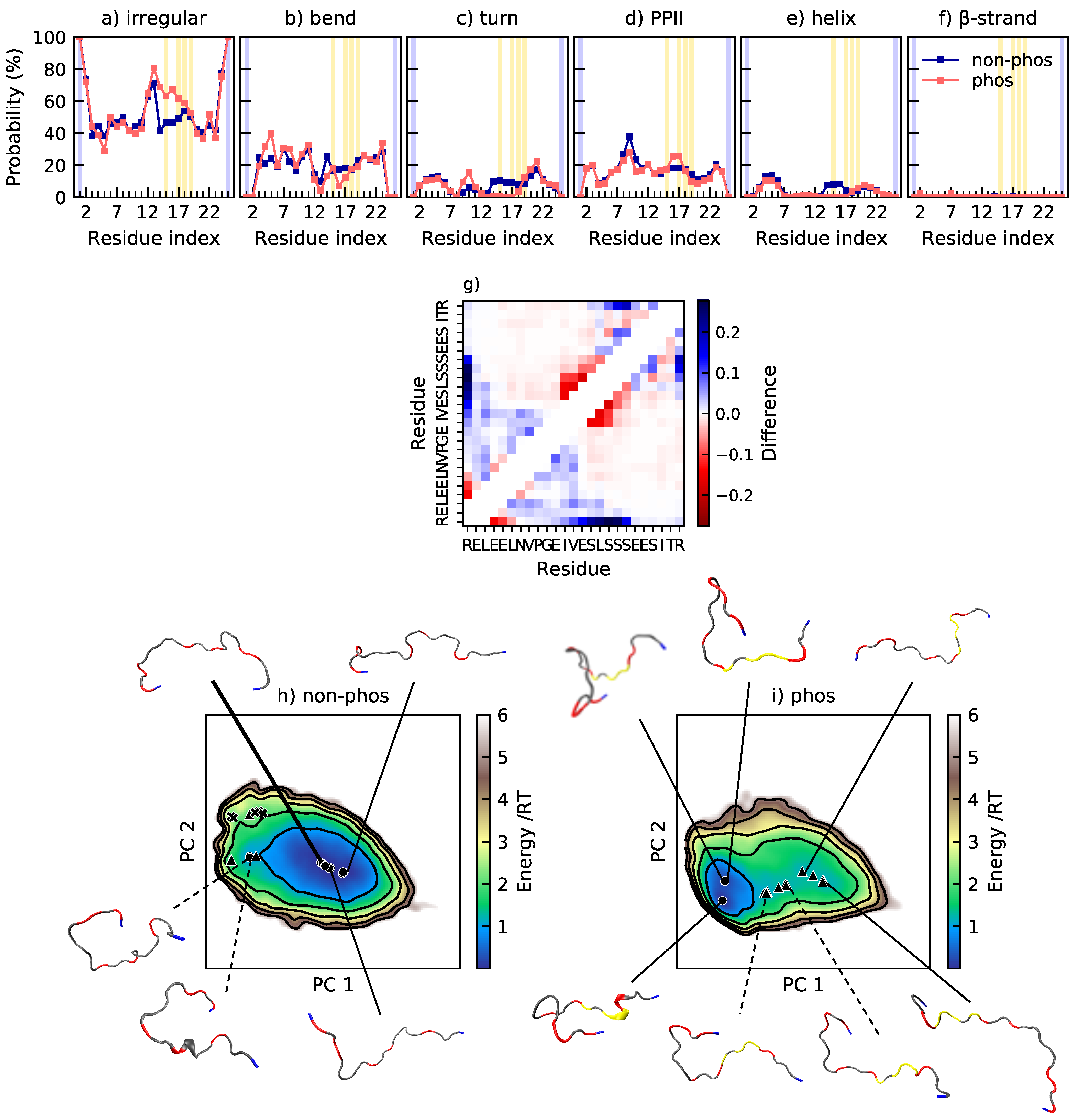
2.2. Phosphorylation of Tau1 Favors Expanded Conformations

Tau1 is dominated by irregular structure and polyproline type II helix (PPII), as shown in Figure 3a–f. It possesses 46% and 51% PPII in the non-phosphorylated and phosphorylated state, respectively. Elam et al. [41] have predicted close to 50% PPII content in this region of Tau, and CD measurements of this segment indicate an increase of PPII content upon phosphorylation [15]. In Figure 3a–f, it is shown that all structural changes upon phosphorylation at T175 and T181 take place at the C-terminal end of the peptide, from residue 179 and forward. The propensity for bends and turns at residue 179–181 decreases, while the PPII content increases at residues 181–182. There is occasional salt bridge formation between the phosphothreonines and their respective neighboring lysine. Specifically, the probability of salt bridge formation is 7 ± 2 % for pT175–K174 and 9 ± 2 % for pT181–K180. The most occurring salt bridge is, however, formed between pT175 and the N-terminal, with a probability of 49 ± 9 %. However, due to the close proximity between the salt bridging residues, the effect on the overall dimensions of the peptide is small. Since Tau1 is a short and rather stiff peptide, as shown by the shape factor in Figure 2, there is limited contact between residues. The change in contact probability upon phosphorylation is also small, according to Figure 3g, which reveals that the main change is a decrease of contact between T181 and the preceding residues A177 and P178, in agreement with the decreased probability of a bend or turn in that region, as shown by Figure 3b,c. The conformational effects of phosphorylation of Tau are well summarized by Figure 3h,i, showing the energy landscape and conformations of non-phosphorylated and phosphorylated Tau1. The energy landscape of non-phosphorylated Tau1 contains several minima, of which the minimum containing expanded conformations dominate, in line with the relatively high shape factor. Other less populated minima contain conformations with a kink in the C-terminal end, originating from a bend or turn. Upon phosphorylation, the minima with kinked conformations disappears, leaving only the minima with expanded conformations. This is in line with decreased contact probability and explains the change in shape of the Rg and Ree distributions, from a peak with a preceding shoulder to a single peak.

2.3. Phosphorylation Increases the Helix Propensity and Induces Salt Bridge Formation in Tau2 and SN15

Tau2 and SN15 are both mainly irregular and report an increase of helicity upon phosphorylation, see Figure 4a–f and Figure 5a–f, respectively. The helical region is identified as “pSpSAKSR” in Tau2 and “pSpSEEKFLR” in SN15, according to Figure 4e and Figure 5e. The sequences, hence, share two characteristics: (1) the helical region starts with two phoshorylation sites, and (2) three or four steps away from the phosphorylation site, a positively charged residue is positioned. Phosphorylation has been shown to stabilize α-helices if the phosphorylation site is located in the N-terminal end of the helix, by electrostatic interaction between phosphorylated serines and the macrodipole of the helix, and by hydrogen bonding with the amide backbone [42]. With a i , i + 4 spacing between a phosphorylated serine and a lysine, phosphorylation also stabilizes α-helices through salt bridge formation between the side groups [43].
For Tau2, a phosphorylation-induced increase of α-helical structure from 5 to 40% in region A239–R242 has been reported [13]. In these simulations, the main helical increase upon phosphorylation is associated with region S237–K240, where the increase is from 4 to 26%. However, the helical increase is mainly due to 310-helix, since the increase of α-helix is only from 1 to 5%. Hence, the simulations are in qualitative agreement with the experiments, but the quantitative results should be treated with caution. In addition, in SN15, the larger part of the helical increase is due to 310-helix, and an increase of α-helix is supported by CD spectroscopy [20], once again giving qualitative support to the findings in this study. Notice also that, while it is hard to make quantitative comparisons with CD data, our study on SN15 suggested that the simulations underestimate the structural content [20], which is the same as observed for Tau2.
While helix formation decreases the Rg and Ree, salt bridge formation can also contribute to the compaction observed upon phosphorylation. In Tau2, several salt bridges have been established from NMR measurements, specifically pT231–R230, pS237–K240, and pS238–R242 [13]. pT231–R230 and pS238–R242 are indeed the two most occurring salt bridges according to Table 3, while pS237–R242 is the third most common. Apart from the increase of helical content related to phosphorylation, Figure 4b reveals an interesting pattern of bends after phosphorylation, where the charged residues R, K, pT, and pS are enriched in bends. The conformations in Figure 4 illustrate how the salt bridges contribute to the formation of bends. Since the probability of a turn at A227–V229 is roughly the same as the probability of the pT231–K225 salt bridge (see Figure 3 and Figure 4c), and V228 is located right between K225 and pT231, we conclude that this turn is also a result of a salt bridge interaction. Hence, this peptide shows that salt bridge formation can induce bends and turns.
Comparing the energy landscapes of non-phosphorylated and phosphorylated Tau2 in Figure 4h,i, it is shown that, for both peptides, more extended conformations, such as in the minima furthest to the right, are sampled, but to a different extent. These type of conformations are more common in the non-phosphorylated variant, while the most populated basin contains conformations with the N-terminal end folded over, to come closer to the phosphorylated residues. While K225 rarely involves in a proper salt bridge with other residues than pT231, it is still energetically favorable to be in rather close vicinity of the phosphorylated region, considering both the charged side chain and the N-terminus. These types of conformations give rise to an increased contact probability within the N-terminal part of the chain, see Figure 4g. The increased contact probability close to the diagonal in the middle to C-terminal end corresponds to the increase of helical structure and certain salt bridges. Apart from those, there is a decrease of the probability of contacts within the C-terminal end upon phosphorylation. The two minima in the left part of the energy landscape of non-phosphorylated Tau2 in Figure 4h are examples of conformations with a higher level of contact within the C-terminal end. They originate from the electrostatic attraction between the C-terminus and the positively charged residues. In phosphorylated Tau2, that region of the energy landscape is visited much less (see Figure 4i), in agreement with the changes in contact probability. Notice, however, that the probability of conformations with one end folded over is much higher after phosphorylation, which explains the decrease in Rg and Ree. The conformation corresponding to the minimum in the most populated basin for the phosphorylated peptide additionally shows a helix in the C-terminal end, which also contributes to a decreased Rg and Ree.
In SN15, the salt bridges pS2–K6, pS3–K6, pS3–R9, and pS3–R10 are the most probable and all form with an approximately 25% occurrence. From the change in contact probability displayed in Figure 5g, it appears that the pS2–K6 and pS3–K6 salt bridges contribute to stabilize the formed helix. The pS3–R9 and pS3–R10 salt bridges are also visible in the contact map and contribute to an increase in the amount of more compact conformations after phosphorylation. In the energy landscape in Figure 5, it is shown that phosphorylation shifts the position of the main minima in the energy landscape, from an area of more coil-like structures to a more compact state. The non-phosphorylated peptide also samples conformations that are more compact with a higher content of secondary structure, but more rarely than the phosphorylated peptide. The conformation corresponding to the minimum in the most populated basin in the phosphorylated peptide has residue pS2 and K6 close enough to be in contact; however, there is no helix, but instead a turn at residues E4–E5. This shows that it is favorable to have pS2 and K6 in contact, but that the interaction does not necessarily imply helix formation. In Figure 5c, it was shown that the turn content in region S3–E5 also increases upon phosphorylation, not only the helix content. There is also an increase of turn content in region F7–R11, which is partly caused by occasional β-strand formation, as shown in the other conformation in Figure 5, and partly by residues pS3 and R9 coming close to form a salt bridge, in line with the turn induced in Tau2. Both of these changes give rise to more compact conformations. We must, however, note that SAXS measurements have indicated that a compaction upon phosphorylation is plausible, but probably smaller than shown in the simulations [20]. While Jin and Gräter found that changes in the hydration shell upon phosphorylation can hide global conformational changes in SAXS measurements, they also concluded that the force field used in this study overestimates the charge effect, thus providing two different explanations of the deviations between the simulations and experiments [10]. Note also that the contact map reports a decrease of contact between R10 and F14, a contact probably formed due to cation–π interaction, which will be discussed further in the section regarding Stath.

2.4. Salt Bridge Formation Shifts the Conformational Ensemble of bCPP

For bCPP, the secondary structure content is dominated by an irregular structure and is highly similar in phosphorylated and non-phosphorylated states, as shown by Figure 6a–f, in agreement with CD spectroscopy results by Farrell et al. [25]. The small difference that occurs upon phosphorylation at S14, S17, S18, and S19 is a change from helix and turn to irregular structure in region E14–S17. The vanishing of helical content is in agreement with the conclusion of Andrew et al. that phosphorylation of a residue in the interior of a helix, without a positively charged residue within suitable distance, destabilizes the helix [42]. Since disruption of a short helix would not cause a contraction of the peptide, the conformational changes in bCPP upon phosphorylation are not explained by secondary structure. Instead, the contraction is due to electrostatic attraction including salt bridge formation between the positively charged end residues and the phosphorylated residues, as seen in Table 4. Although both end residues are arginines, there is a preference of R1 to interact with the phosphorylated region over R25, due to the respective charges of the termini. This is evident from the fact that the N-terminus is also involved in salt bridges with the phosphorylated residues, and further shown by the difference in contact probability in Figure 6g. When R1 interacts with the phosphorylated residues, it causes the peptide to fold over, reducing Rg and Ree substantially. From the energy landscapes in Figure 6h,i, it is shown that before phosphorylation the minima with lowest energy contain more extended conformations, while after phosphorylation the minima with lowest energy instead showcase the N-terminal part being folded over.
Based only on the net charge of non-phosphorylated bCPP, it was expected that it would expand upon phosphorylation. Considering only region E13–E21, which contains the four phosphorylation sites, this effect was noticed. The average distance between the C atoms of residue 13 and 21 increases from 1.91 ± 0.03 nm to 2.12 ± 0.03 nm upon phosphorylation. However, due to the strong electrostatic interaction between the arginines and the phosphorylated region that are far apart in the sequence, the global result is compaction. Hence, the relative position of charged residues is very important to consider for the effects of phosphorylation on the overall dimensions of the peptide.
We previously showed that the addition of 150 mM NaCl had negligible effects on the salt bridges and global conformational properties of phosphorylated bCPP [31]. The same applies to non-phosphorylated bCPP, as presented in Supplementary File S1, Figures S1 and S2. However, although the average values of Rg at 0 and 150 mM are within error, there is a slight increase in the phosphorylated variant and decrease in the non-phosphorylated variant, see Table 5. Hence, at 150 mM NaCl, the difference observed in Rg between the two variants vanishes, considering the associated error. Note, however, that the distributions still have distinctly different shapes, hence we argue that the conformational ensembles are still different. The same trend is observed in the average Ree values, although a difference with respect to phosphorylation state still remains at 150 mM NaCl, see Table 5. In addition, in the calculated scattering curve (Supplementary File S1, Figure S2), the effect of salt is smaller than the effect of phosphorylation. The difference between the form factor of non-phosphorylated and phosphorylated bCPP is, however, still rather small, so we suspect that it can be hard to detect experimentally with SAXS. Based on the fraction of charged residues and level of charge separation, we expect the other peptides in this study to show smaller effects in regard to salt concentration than bCPP. Hence, we expect the results observed here to be also valid at 150 mM NaCl.

2.5. Arginine—Phosphoserine Interactions Outshines Arginine—Tyrosine Interactions in Stath

Upon phosphorylation of Stath, the three largest changes in secondary structure are a decrease of β-strand structure, an increase of helical structure, and an increase of turns, according to Figure 7a–f. The increase of helical structure is in the same region as observed for the N-terminal fragment SN15. Figure 7f implies that residues R10, Y18, Y21, and Y41 are of extra importance for the formation of β-sheet. The cation–π interaction that can occur between aromatic residues, such as tyrosine, and cationic residues, such as arginine, have been shown to be common in proteins [44]. A correlation between β-strands and cation–π interactions have also been established [45]. Table 6 show that the cation–π interaction indeed is more occurring in non-phosphorylated Stath than in phosphorylated Stath, suggesting that it drives the formation of β-strands. The conformations in Figure 7I–III show examples of the cation–π interaction in non-phosphorylated Stath. Although the aromatic–cation interactions are more common in non-phosphorylated Stath, they still occur in phosphorylated Stath, as exemplified by Figure 7. Upon phosphorylation, the occurrence of cation–π interaction decreases substantially, while salt bridge formation appears according to Table 7. Notice that R10, which was shown to interact with tyrosines, is involved in one of the most probable salt bridges, pS3–R10. Hence, the arginine–phosphoserine interaction is deemed stronger than the arginine–tyrosine interaction. The replacement of arginine–tyrosine interaction with arginine–phosphoserine causes the β-strands to vanish, which explains the observed expansion.
As presented above, SN15, which is the first fifteen residues of Stath, contracts upon phosphorylation, which was explained by the increased helicity and formation of salt bridges. Supplementary File S1, Figure S3 shows that, in phosphorylated Stath, the global dimensions of the first fifteen residues, Stath1–15 agree with those of the fragment (SN15). In the non-phosphorylated variant, the distributions are also rather similar, except for a sharp peak in both the Rg and Ree distributions, which corresponds to a basin in the energy landscape with the conformation shown in Supplementary File S1, Figure S3c. Regarding the secondary structure, according to Supplementary File S1, Figure S4, the largest difference between SN15 and Stath1–15 is caused by β-strand not forming in SN15, due to lacking its partner further on in the sequence. There are also some differences in bends and turns, but the increase of helical propensity is similar. Hence, overall, the first fifteen residues of Stath behave rather similarly in the full peptide and as a standalone fragment, although especially the presence of the rest of the sequence induces β-strand formation. Despite this discrepancy, we can conclude that phosphorylation of Stath causes a contraction of the first fifteen residues, but an expansion of the full peptide, due to disruption of β-sheets.

3. Conclusions

Some of the peptides in this study contracted upon phosphorylation, while others became more expanded. However, the net charge was not enough to predict the effect in these short peptides. Instead, we have identified factors that appeared to be of greater importance, of which the first is the distribution of charged residues, in line with the influence of linear charge distribution on the conformational ensemble of IDPs [46]. Especially the relative position of phosphorylated and positively charged residues mattered, considering that salt bridges formed between residues far from each other in the sequence had the largest effect on the overall dimensions of the peptide. Regarding salt bridges, Kumar et al. have shown that phosphorylation can re-wire salt bridges by competing with already present E–R salt bridges [47], but no such tendencies were observed for these peptides. Here, the possible salt bridges in the non-phosphorylated peptides were either low in probability or did not change much upon phosphorylation. In Stath, competitive interactions between positively charged residues, aromatic residues, and phosphorylated residues accounted for the changes upon phosphorylation. This shows that, for peptides which include arginine, it can be of importance to also consider aromatic residues. In both bCPP and Stath, phosphorylation induced the opposite effect on the local and global dimensions, hence, to understand the purpose/implications of the phosphorylated residues, both length-scales should be studied. This is especially important dealing with longer IDPs where local/non-local effects can have larger compensatory effect than observed for short peptides [14].
Regarding secondary structure, the separation between phosphorylated and positively charged residues was shown to control the helix propensity, and salt bridges additionally induced changes in the amount of bends and turns. Comparison with experimental data on secondary structure for SN15 and Tau2 indicates that the simulations underestimate the structural content. For these peptides, a preference of 310- over α-helix was also observed, while the experimental data only considered α-helix. Hence, the simulations were better at indicating trends than producing exact measurements of secondary structure. Overall, the simulation results were often in qualitative agreement with available experimental data, suggesting that, despite the deficiency related to secondary structure and the reported tendency of the force field to overestimate charge–charge interactions, simulations with this force field can still contribute to an increased understanding of the implications of phosphorylation.
As a final note, this study shows that there are several factors contributing to the outcome of phosphorylation, and that they are of varying importance in different peptides. This shows that phosphorylation indeed is complex; however, it is still possible to obtain a better understanding of these factors individually. Therefore, we have an ongoing project in which the number of phosphorylated residues and their positions are varied in a controlled manner, to investigate the effects of those factors systematically.

4. Materials and Methods

All-atom molecular dynamics simulations of the systems shown in Table 8 were performed using GROMACS version 2018.4 (version 4.6.7 for simulation of Stathn) [48,49,50,51,52] with the AMBER ff99SB-ILDN [53] force field and the TIP4P-D [54] water model. Parameters for phosphorylated residues were derived from Homeyer et al. [55] and Steinbrecher et al. [56]. Please note that some of the data sets are previously published and only re-analyzed for this study.
Initial configurations of the peptides were constructed from the sequence as linear chains using Avogadro 1.2.0 [57], optimizing the structure with the auto-optimization tool. SN15n and Stathn were constructed as linear chains in PyMOL [58]. Each peptide was placed in a rhombic dodecahedron box with a minimum distance between the peptide and the box edges of 1 nm, and solvated. The number of water molecules is specified in Table 8, alongside the number of chloride and sodium ions that were added to neutralize the system and in two cases obtain a salt concentration of 150 mM. Periodic boundary conditions were employed in all directions. The equations of motion were integrated using the Verlet leapfrog algorithm [59] with a time step of 2 fs. Non-bonded interactions were treated with a Verlet list cutoff scheme. The short-ranged interactions were calculated using neighbor lists with a cutoff of 1 nm. Long-ranged dispersion corrections were applied to energy and pressure and long-ranged electrostatic interactions were treated by Particle Mesh Ewald [60] with a cubic interpolation and 0.16 nm grid spacing. All bond lengths were constrained using the LINCS algorithm [61]. Solute and solvent were separately coupled to temperature baths at 298 K using the velocity rescaling thermostat [62] with a 0.1 ps relaxation time. Parrinello–Raman pressure coupling [63] was used to keep the pressure at 1 bar, using a 2 ps relaxation time and 4.5 · 10 5 bar-1 isothermal compressibility.
Energy minimization was performed by the steepest descent algorithm until the system was converged within the available machine precision. Initiation of five replicates per system with different starting seeds were performed separately in two steps using position restraints on the peptide. The first step was 500 ps of NVT simulation (constant number of particles, volume, and temperature) performed to stabilize the temperature, followed by the second step of 1000 ps of NPT simulation (constant number of particles, pressure, and temperature) to stabilize the pressure. Production runs of the five replicates per system were performed in the NPT ensemble, for at least 1 µs per replicate. bCPPp with 150 mM salt was simulated in 10 replicates for 0.7 µs each. The total simulation time per system is stated in Table 8. Energies and coordinates were saved every 10 ps, except for in the simulations with 150 mM NaCl. The saving frequency there was every 50 or 40 ps, for bCPPn and bCPPp, respectively.

Analysis

Rg and Ree were calculated using GROMACS 2018.4 and the gmx analyze routine was used to obtain averages and error estimates from block averaging analysis. Distributions were obtained by Gaussian kernel estimation using the SciPy package version 1.5.4 [64]. The shape factor, r s , was calculated from the average values of Rg and Ree according to:
r s = R ee 2 R g 2 .
Secondary structure was determined using the DSSP program version 2.2.1 [65] with an extension to detect polyproline type II structure [66,67], on 10,000 equally spaced frames from the combined trajectory. The MDTraj Python library version 1.9.3 [68] was used to obtain contact maps, analyze salt bridges, and cation–π interactions. For the contact maps, contact was defined as when two atoms of different residues were within 0.4 nm of each other. Since salt bridges are formed as a result of hydrogen bonding and electrostatic interactions, they have been assessed by analyzing the presence of hydrogen bonds based on the criterion in reference [69], as implemented in MDTraj. Cation– interactions were analyzed based on the position of the NZ atom in arginine and CG and CZ in tyrosine. Interaction was defined to occur when both the distances R:NZ–Y:CG and R:NZ–Y:CZ were ≤0.6 nm [44]. The energy landscapes were calculated using principal component analysis following the approach described by Campos and Baptista [70], with the differences described by Henriques et al. [71]. In short, principal component analysis was applied to the Cartesian coordinates of the backbone atoms of the protein, obtained after translational and rotational least square fitting on the central structure of the simulation. The conditional free energy was calculated from the probability density function in the representation space constructed by the first two principal components, obtained by Gaussian kernel density estimation. Snapshots from the simulations were produced using VMD 1.9.3 [72,73,74]. Data were plotted using a Jupyter Notebook [75] with Python version 3.6.4 and packages NumPy version 1.19.5 [76] and Matplotlib version 2.1.2 [77].
Convergence and sampling quality were assessed by comparing the Rg and Ree distributions, and energy landscapes, between the replicates, as well as by observing the auto-correlation function and convergence of the block average error estimate of Rg and Ree in the concatenated simulation. These data are available in Supplementary File S2.

Supplementary Materials

The following are available online at https://www.mdpi.com/article/10.3390/ijms222011058/s1.

Author Contributions

Conceptualization, M.S. and E.R.; data curation, E.R.; formal analysis, M.S. and E.R.; funding acquisition, M.S.; investigation, E.R.; methodology, M.S. and E.R.; project administration, M.S. and E.R.; resources, M.S.; supervision, M.S.; validation, M.S. and E.R.; visualization, M.S. and E.R.; writing—original draft, E.R.; writing—review and editing, M.S. and E.R. All authors have read and agreed to the published version of the manuscript.

Funding

Financial support has been given by the Royal Physiographic Society in Lund and the Bertil Andersson foundation.

Institutional Review Board Statement

Not applicable.

Informed Consent Statement

Not applicable.

Data Availability Statement

Data are included in the article or Supplementary Material.

Acknowledgments

The simulations were performed on resources provided by the Swedish National Infrastructure for Computing (SNIC) at the Center for Scientific and Technical Computing at Lund University (LUNARC).

Conflicts of Interest

The authors declare no conflict of interest.

Abbreviations

The following abbreviations are used in this manuscript:
IDPIntrinsically disordered protein
CDCircular dichroism
NMRNuclear magnetic resonance
RgRadius of gyration
ReeEnd-to-end distance
SAXSSmall-angle X-ray scattering

References

  1. Dunker, A.; Lawson, J.; Brown, C.J.; Williams, R.M.; Romero, P.; Oh, J.S.; Oldfield, C.J.; Campen, A.M.; Ratliff, C.M.; Hipps, K.W.; et al. Intrinsically disordered protein. J. Mol. Graph. Model. 2001, 19, 26–59. [Google Scholar] [CrossRef] [Green Version]
  2. Tompa, P. Intrinsically unstructured proteins. Trends Biochem. Sci. 2002, 27, 527–533. [Google Scholar] [CrossRef]
  3. Fisher, C.K.; Stultz, C.M. Constructing ensembles for intrinsically disordered proteins. Curr. Opin. Struct. Biol. 2011, 21, 426–431. [Google Scholar] [CrossRef] [PubMed] [Green Version]
  4. Uversky, V.N. Wrecked regulation of intrinsically disordered proteins in diseases: Pathogenicity of deregulated regulators. Front. Mol. Biosci. 2014, 1, 6. [Google Scholar] [CrossRef] [PubMed]
  5. Babu, M.M.; van der Lee, R.; de Groot, N.S.; Gsponer, J. Intrinsically disordered proteins: Regulation and disease. Curr. Opin. Struct. Biol. 2011, 21, 432–440. [Google Scholar] [CrossRef] [PubMed]
  6. Dunker, A.K.; Brown, C.J.; Lawson, J.D.; Iakoucheva, L.M.; Obradovićá, Z. Intrinsic Disorder and Protein Function. Biochemistry 2002, 41, 6573–6582. [Google Scholar] [CrossRef] [Green Version]
  7. Iakoucheva, L.M.; Radivojac, P.; Brown, C.J.; O’Connor, T.R.; Sikes, J.G.; Obradovic, Z.; Dunker, A.K. The importance of intrinsic disorder for protein phosphorylation. Nucleic Acids Res. 2004, 32, 1037–1049. [Google Scholar] [CrossRef] [Green Version]
  8. Gao, J.; Xu, D. Correlation Between Posttranslational Modification and Intrinsic Disorder in Protein. In Biocomputing 2012; Altman, R.B., Dunker, A.K., Hunter, L., Murray, T.A., Klein, T.E., Eds.; World Scientific Publishing Co. Pte. Ltd.: Singapore, 2012; pp. 94–103. [Google Scholar] [CrossRef] [Green Version]
  9. Johnson, L.N.; Lewis, R.J. Structural Basis for Control by Phosphorylation. Chem. Rev. 2001, 101, 2209–2242. [Google Scholar] [CrossRef]
  10. Jin, F.; Gräter, F. How multisite phosphorylation impacts the conformations of intrinsically disordered proteins. PLoS Comput. Biol. 2021, 17, e1008939. [Google Scholar] [CrossRef] [PubMed]
  11. Firman, T.; Ghosh, K. Sequence charge decoration dictates coil-globule transition in intrinsically disordered proteins. J. Chem. Phys. 2018, 148, 123305. [Google Scholar] [CrossRef]
  12. Uversky, V.N. Intrinsically Disordered Proteins and Their “Mysterious” (Meta)Physics. Front. Phys. 2019, 7, 10. [Google Scholar] [CrossRef] [Green Version]
  13. Schwalbe, M.; Kadavath, H.; Biernat, J.; Ozenne, V.; Blackledge, M.; Mandelkow, E.; Zweckstetter, M. Structural Impact of Tau Phosphorylation at Threonine 231. Structure 2015, 23, 1448–1458. [Google Scholar] [CrossRef] [PubMed] [Green Version]
  14. Martin, E.W.; Holehouse, A.S.; Grace, C.R.; Hughes, A.; Pappu, R.V.; Mittag, T. Sequence Determinants of the Conformational Properties of an Intrinsically Disordered Protein Prior to and upon Multisite Phosphorylation. J. Am. Chem. Soc. 2016, 138, 15323–15335. [Google Scholar] [CrossRef] [PubMed] [Green Version]
  15. Chin, A.F.; Toptygin, D.; Elam, W.A.; Schrank, T.P.; Hilser, V.J. Phosphorylation Increases Persistence Length and End-to-End Distance of a Segment of Tau Protein. Biophys. J. 2016, 110, 362–371. [Google Scholar] [CrossRef] [PubMed] [Green Version]
  16. Kulkarni, P.; Jolly, M.K.; Jia, D.; Mooney, S.M.; Bhargava, A.; Kagohara, L.T.; Chen, Y.; Hao, P.; He, Y.; Veltri, R.W.; et al. Phosphorylation-induced conformational dynamics in an intrinsically disordered protein and potential role in phenotypic heterogeneity. Proc. Natl. Acad. Sci. USA 2017, 114, E2644–E2653. [Google Scholar] [CrossRef] [Green Version]
  17. Wang, K.; Ning, S.; Guo, Y.; Duan, M.; Yang, M. The regulation mechanism of phosphorylation and mutations in intrinsically disordered protein 4E-BP2. Phys. Chem. Chem. Phys. 2020, 22, 2938–2948. [Google Scholar] [CrossRef]
  18. Rani, L.; Mittal, J.; Mallajosyula, S.S. Effect of Phosphorylation and O-GlcNAcylation on Proline-Rich Domains of Tau. J. Phys. Chem. B 2020, 124, 1909–1918. [Google Scholar] [CrossRef]
  19. Liu, N.; Guo, Y.; Ning, S.; Duan, M. Phosphorylation regulates the binding of intrinsically disordered proteins via a flexible conformation selection mechanism. Commun. Chem. 2020, 3, 123. [Google Scholar] [CrossRef]
  20. Rieloff, E.; Skepö, M. Phosphorylation of a Disordered Peptide—Structural Effects and Force Field Inconsistencies. J. Chem. Theory Comput. 2020, 16, 1924–1935. [Google Scholar] [CrossRef]
  21. Willet, A.H.; Igarashi, M.G.; Chen, J.S.; Bhattacharjee, R.; Ren, L.; Cullati, S.N.; Elmore, Z.C.; Roberts-Galbraith, R.H.; Johnson, A.E.; Beckley, J.R.; et al. Phosphorylation in the intrinsically disordered region of F-BAR protein Imp2 regulates its contractile ring recruitment. J. Cell Sci. 2021, 134. [Google Scholar] [CrossRef] [PubMed]
  22. Papamokos, G.V.; Tziatzos, G.; Papageorgiou, D.G.; Georgatos, S.; Kaxiras, E.; Politou, A.S. Progressive Phosphorylation Modulates the Self-Association of a Variably Modified Histone H3 Peptide. Front. Mol. Biosci. 2021, 8, 558. [Google Scholar] [CrossRef] [PubMed]
  23. Nicolaou, S.T.; Hebditch, M.; Jonathan, O.J.; Verma, C.S.; Warwicker, J. PhosIDP: A web tool to visualize the location of phosphorylation sites in disordered regions. Sci. Rep. 2021, 11, 9930. [Google Scholar] [CrossRef] [PubMed]
  24. Mittag, T.; Marsh, J.; Grishaev, A.; Orlicky, S.; Lin, H.; Sicheri, F.; Tyers, M.; Forman-Kay, J.D. Structure/Function Implications in a Dynamic Complex of the Intrinsically Disordered Sic1 with the Cdc4 Subunit of an SCF Ubiquitin Ligase. Structure 2010, 18, 494–506. [Google Scholar] [CrossRef] [PubMed] [Green Version]
  25. Farrell, H.; Qi, P.; Wickham, E.; Unruh, J. Secondary Structural Studies of Bovine Caseins: Structure and Temperature Dependence of β-Casein Phosphopeptide (1–25) as Analyzed by Circular Dichroism, FTIR Spectroscopy, and Analytical Ultracentrifugation. J. Protein Chem. 2002, 21, 307–321. [Google Scholar] [CrossRef] [PubMed]
  26. Brister, M.A.; Pandey, A.K.; Bielska, A.A.; Zondlo, N.J. OGlcNAcylation and Phosphorylation Have Opposing Structural Effects in tau: Phosphothreonine Induces Particular Conformational Order. J. Am. Chem. Soc. 2014, 136, 3803–3816. [Google Scholar] [CrossRef] [PubMed]
  27. Chong, S.H.; Chatterjee, P.; Ham, S. Computer Simulations of Intrinsically Disordered Proteins. Annu. Rev. Phys. Chem. 2017, 68, 117–134. [Google Scholar] [CrossRef]
  28. Huang, J.; MacKerell, A.D., Jr. Force field development and simulations of intrinsically disordered proteins. Curr. Opin. Struct. Biol. 2018, 48, 40–48. [Google Scholar] [CrossRef]
  29. Ahmed, M.C.; Papaleo, E.; Lindorff-Larsen, K. How well do force fields capture the strength of salt bridges in proteins? PeerJ 2018, 6, e4967. [Google Scholar] [CrossRef]
  30. Piana, S.; Lindorff-Larsen, K.; Shaw, D.E. How Robust Are Protein Folding Simulations with Respect to Force Field Parameterization? Biophys. J. 2011, 100, L47–L49. [Google Scholar] [CrossRef] [Green Version]
  31. Rieloff, E.; Skepö, M. Molecular Dynamics Simulations of Phosphorylated Intrinsically Disordered Proteins: A Force Field Comparison. Int. J. Mol. Sci. 2021, 22, 10174. [Google Scholar] [CrossRef]
  32. Cleveland, D.W.; Hwo, S.Y.; Kirschner, M.W. Purification of tau, a microtubule-associated protein that induces assembly of microtubules from purified tubulin. J. Mol. Biol. 1977, 116, 207–225. [Google Scholar] [CrossRef]
  33. Buée, L.; Bussière, T.; Buée-Scherrer, V.; Delacourte, A.; Hof, P.R. Tau protein isoforms, phosphorylation and role in neurodegenerative disorders11These authors contributed equally to this work. Brain Res. Rev. 2000, 33, 95–130. [Google Scholar] [CrossRef]
  34. Gong, C.X.; Iqbal, K. Hyperphosphorylation of microtubule-associated protein tau: A promising therapeutic target for Alzheimer disease. Curr. Med. Chem. 2008, 15, 2321–2328. [Google Scholar] [CrossRef]
  35. Hay, D.; Smith, D.; Schluckebier, S.; Moreno, E. Basic Biological Sciences Relationship between Concentration of Human Salivary Statherin and Inhibition of Calcium Phosphate Precipitation in Stimulated Human Parotid Saliva. J. Dent. Res. 1984, 63, 857–863. [Google Scholar] [CrossRef]
  36. Moreno, E.; Zahradnik, R. Demineralization and Remineralization of Dental Enamel. J. Dent. Res. 1979, 58, 896–903. [Google Scholar] [CrossRef] [PubMed]
  37. Raj, P.A.; Johnsson, M.; Levine, M.J.; Nancollas, G.H. Salivary statherin. Dependence on sequence, charge, hydrogen bonding potency, and helical conformation for adsorption to hydroxyapatite and inhibition of mineralization. J. Biol. Chem. 1992, 267, 5968–5976. [Google Scholar] [CrossRef]
  38. Holt, C.; Timmins, P.A.; Errington, N.; Leaver, J. A core-shell model of calcium phosphate nanoclusters stabilized by β-casein phosphopeptides, derived from sedimentation equilibrium and small-angle X-ray and neutron-scattering measurements. Eur. J. Biochem. 1998, 252, 73–78. [Google Scholar] [CrossRef]
  39. Little, E.M.; Holt, C. An equilibrium thermodynamic model of the sequestration of calcium phosphate by casein phosphopeptides. Eur. Biophys. J. 2004, 33, 435–447. [Google Scholar] [CrossRef]
  40. Ferraretto, A.; Gravaghi, C.; Fiorilli, A.; Tettamanti, G. Casein-derived bioactive phosphopeptides: Role of phosphorylation and primary structure in promoting calcium uptake by HT-29 tumor cells. FEBS Lett. 2003, 551, 92–98. [Google Scholar] [CrossRef] [Green Version]
  41. Austin Elam, W.; Schrank, T.P.; Campagnolo, A.J.; Hilser, V.J. Evolutionary conservation of the polyproline II conformation surrounding intrinsically disordered phosphorylation sites. Protein Sci. 2013, 22, 405–417. [Google Scholar] [CrossRef] [Green Version]
  42. Andrew, C.D.; Warwicker, J.; Jones, G.R.; Doig, A.J. Effect of Phosphorylation on α-Helix Stability as a Function of Position. Biochemistry 2002, 41, 1897–1905. [Google Scholar] [CrossRef]
  43. Errington, N.; Doig, A.J. A Phosphoserine-Lysine Salt Bridge within an α-Helical Peptide, the Strongest α-Helix Side-Chain Interaction Measured to Date. Biochemistry 2005, 44, 7553–7558. [Google Scholar] [CrossRef]
  44. Gallivan, J.P.; Dougherty, D.A. Cation-π interactions in structural biology. Proc. Natl. Acad. Sci. USA 1999, 96, 9459–9464. [Google Scholar] [CrossRef] [Green Version]
  45. Tayubi, I.; Sethumadhavan, R. Nature of cation-π interactions and their role in structural stability of immunoglobulin proteins. Biochemistry 2010, 75, 912–918. [Google Scholar] [CrossRef]
  46. Das, R.K.; Pappu, R.V. Conformations of intrinsically disordered proteins are influenced by linear sequence distributions of oppositely charged residues. Proc. Natl. Acad. Sci. USA 2013, 110, 13392–13397. [Google Scholar] [CrossRef] [Green Version]
  47. Kumar, P.; Chimenti, M.S.; Pemble, H.; Schönichen, A.; Thompson, O.; Jacobson, M.P.; Wittmann, T. Multisite Phosphorylation Disrupts Arginine-Glutamate Salt Bridge Networks Required for Binding of Cytoplasmic Linker-associated Protein 2 (CLASP2) to End-binding Protein 1 (EB1) *. J. Biol. Chem. 2012, 287, 17050–17064. [Google Scholar] [CrossRef] [PubMed] [Green Version]
  48. Berendsen, H.; van der Spoel, D.; van Drunen, R. GROMACS: A message-passing parallel molecular dynamics implementation. Comput. Phys. Commun. 1995, 91, 43–56. [Google Scholar] [CrossRef]
  49. Hess, B.; Kutzner, C.; van der Spoel, D.; Lindahl, E. GROMACS 4: Algorithms for Highly Efficient, Load-Balanced, and Scalable Molecular Simulation. J. Chem. Theory Comput. 2008, 4, 435–447. [Google Scholar] [CrossRef] [Green Version]
  50. Pronk, S.; Páll, S.; Schulz, R.; Larsson, P.; Bjelkmar, P.; Apostolov, R.; Shirts, M.R.; Smith, J.C.; Kasson, P.M.; van der Spoel, D.; et al. GROMACS 4.5: A high-throughput and highly parallel open source molecular simulation toolkit. Bioinformatics 2013, 29, 845–854. [Google Scholar] [CrossRef] [PubMed]
  51. Páll, S.; Abraham, M.J.; Kutzner, C.; Hess, B.; Lindahl, E. Tackling Exascale Software Challenges in Molecular Dynamics Simulations with GROMACS. In Solving Software Challenges for Exascale; Markidis, S., Laure, E., Eds.; Springer International Publishing: Cham, Switzerland, 2015; pp. 3–27. [Google Scholar]
  52. Abraham, M.J.; Murtola, T.; Schulz, R.; Páll, S.; Smith, J.C.; Hess, B.; Lindahl, E. GROMACS: High performance molecular simulations through multi-level parallelism from laptops to supercomputers. SoftwareX 2015, 1–2, 19–25. [Google Scholar] [CrossRef] [Green Version]
  53. Lindorff-Larsen, K.; Piana, S.; Palmo, K.; Maragakis, P.; Klepeis, J.L.; Dror, R.O.; Shaw, D.E. Improved side-chain torsion potentials for the Amber ff99SB protein force field. Proteins 2010, 78, 1950–1958. [Google Scholar] [CrossRef] [Green Version]
  54. Piana, S.; Donchev, A.G.; Robustelli, P.; Shaw, D.E. Water Dispersion Interactions Strongly Influence Simulated Structural Properties of Disordered Protein States. J. Phys. Chem. B 2015, 119, 5113–5123. [Google Scholar] [CrossRef]
  55. Homeyer, N.; Horn, A.H.C.; Lanig, H.; Sticht, H. AMBER force-field parameters for phosphorylated amino acids in different protonation states: Phosphoserine, phosphothreonine, phosphotyrosine, and phosphohistidine. J. Mol. Model. 2006, 12, 281–289. [Google Scholar] [CrossRef]
  56. Steinbrecher, T.; Latzer, J.; Case, D.A. Revised AMBER Parameters for Bioorganic Phosphates. J. Chem. Theory Comput. 2012, 8, 4405–4412. [Google Scholar] [CrossRef] [Green Version]
  57. Hanwell, M.D.; Curtis, D.E.; Lonie, D.C.; Vandermeersch, T.; Zurek, E.; Hutchison, G.R. Avogadro: An advanced semantic chemical editor, visualization, and analysis platform. J. Cheminform. 2012, 4, 17. [Google Scholar] [CrossRef] [PubMed] [Green Version]
  58. Schrödinger, L.L.C. The PyMOL Molecular Graphics System; Version 1.2r1. 2009. Available online: https://pymol.org/2/ (accessed on 10 September 2021).
  59. Hockney, R.W.; Eastwood, J.W. Computer Simulation Using Particles; McGraw-Hill: New York, NY, USA, 1981. [Google Scholar]
  60. Darden, T.; York, D.; Pedersen, L. Particle mesh Ewald: An N·log(N) method for Ewald sums in large systems. J. Chem. Phys. 1993, 98, 10089–10092. [Google Scholar] [CrossRef] [Green Version]
  61. Hess, B.; Bekker, H.; Berendsen, H.J.C.; Fraaije, J.G.E.M. LINCS: A linear constraint solver for molecular simulations. J. Comput. Chem. 1997, 18, 1463–1472. [Google Scholar] [CrossRef]
  62. Bussi, G.; Donadio, D.; Parrinello, M. Canonical sampling through velocity rescaling. J. Chem. Phys. 2007, 126, 014101. [Google Scholar] [CrossRef] [PubMed] [Green Version]
  63. Parrinello, M.; Rahman, A. Polymorphic transitions in single crystals: A new molecular dynamics method. J. Appl. Phys. 1981, 52, 7182–7190. [Google Scholar] [CrossRef]
  64. Virtanen, P.; Gommers, R.; Oliphant, T.E.; Haberland, M.; Reddy, T.; Cournapeau, D.; Burovski, E.; Peterson, P.; Weckesser, W.; Bright, J.; et al. SciPy 1.0: Fundamental Algorithms for Scientific Computing in Python. Nat. Methods 2020, 17, 261–272. [Google Scholar] [CrossRef] [Green Version]
  65. Kabsch, W.; Sander, C. Dictionary of protein secondary structure: Pattern recognition of hydrogen-bonded and geometrical features. Biopolymers 1983, 22, 2577–2637. [Google Scholar] [CrossRef] [PubMed]
  66. Mansiaux, Y.; Joseph, A.P.; Gelly, J.C.; de Brevern, A.G. Assignment of PolyProline II Conformation and Analysis of Sequence—Structure Relationship. PLoS ONE 2011, 6, e18401. [Google Scholar] [CrossRef] [PubMed]
  67. Chebrek, R.; Leonard, S.; de Brevern, A.G.; Gelly, J.C. PolyprOnline: Polyproline helix II and secondary structure assignment database. Database 2014, 2014, bau102. [Google Scholar] [CrossRef] [PubMed] [Green Version]
  68. McGibbon, R.T.; Beauchamp, K.A.; Harrigan, M.P.; Klein, C.; Swails, J.M.; Hernández, C.X.; Schwantes, C.R.; Wang, L.P.; Lane, T.J.; Pande, V.S. MDTraj: A Modern Open Library for the Analysis of Molecular Dynamics Trajectories. Biophys. J. 2015, 109, 1528–1532. [Google Scholar] [CrossRef] [PubMed] [Green Version]
  69. Wernet, P.; Nordlund, D.; Bergmann, U.; Cavalleri, M.; Odelius, M.; Ogasawara, H.; Näslund, L.Å.; Hirsch, T.K.; Ojamäe, L.; Glatzel, P.; et al. The Structure of the First Coordination Shell in Liquid Water. Science 2004, 304, 995–999. [Google Scholar] [CrossRef] [Green Version]
  70. Campos, S.R.R.; Baptista, A.M. Conformational Analysis in a Multidimensional Energy Landscape: Study of an Arginylglutamate Repeat. J. Phys. Chem. B 2009, 113, 15989–16001. [Google Scholar] [CrossRef] [PubMed]
  71. Henriques, J.; Cragnell, C.; Skepö, M. Molecular Dynamics Simulations of Intrinsically Disordered Proteins: Force Field Evaluation and Comparison with Experiment. J. Chem. Theory Comput. 2015, 11, 3420–3431. [Google Scholar] [CrossRef] [PubMed]
  72. Humphrey, W.; Dalke, A.; Schulten, K. VMD—Visual Molecular Dynamics. J. Mol. Graph. 1996, 14, 33–38. [Google Scholar] [CrossRef]
  73. Stone, J. An Efficient Library for Parallel Ray Tracing and Animation. Master’s Thesis, Computer Science Department, University of Missouri-Rolla, Rolla, MO, USA, 1998. [Google Scholar]
  74. Frishman, D.; Argos, P. Knowledge-based secondary structure assignment. Proteins 1995, 23, 566–579. [Google Scholar] [CrossRef]
  75. Kluyver, T.; Ragan-Kelley, B.; Pérez, F.; Granger, B.; Bussonnier, M.; Frederic, J.; Kelley, K.; Hamrick, J.; Grout, J.; Corlay, S.; et al. Jupyter Notebooks—A Publishing Format for Reproducible Computational Workflows. In Positioning and Power in Academic Publishing: Players, Agents and Agendas; Loizides, F., Schmidt, B., Eds.; IOS Press: Amsterdam, The Netherlands, 2016; pp. 87–90. [Google Scholar]
  76. Harris, C.R.; Millman, K.J.; van der Walt, S.J.; Gommers, R.; Virtanen, P.; Cournapeau, D.; Wieser, E.; Taylor, J.; Berg, S.; Smith, N.J.; et al. Array programming with NumPy. Nature 2020, 585, 357–362. [Google Scholar] [CrossRef]
  77. Hunter, J.D. Matplotlib: A 2D Graphics Environment. Comput. Sci. Eng. 2007, 9, 90–95. [Google Scholar] [CrossRef]
Figure 1. Radius of gyration (Rg) and end-to-end distance (Ree) density distributions of the non-phosphorylated (non-phos) and phosphorylated (phos) variants. The SN15 data are obtained from Ref. [20] (2020 American Chemical Society), and data for the phosphorylated variants of Tau2, bCPP, and Stath from [31].
Ijms 22 11058 g001
Figure 2. The shape factor of the non-phosphorylated (non-phos) and phosphorylated (phos) variants. The dashed line corresponds to the shape factor of a Gaussian coil. The error bars are based on error propagation of the error estimates determined for radius of gyration and end-to-end distance by block averaging.
Ijms 22 11058 g002
Figure 3. (af) Secondary structure content along the non-phosphorylated and phosphorylated sequence of Tau1. The helix includes α-helix and 310-helix. β-strand also includes β-bridge. The positions of phosphorylated and positively charged residues are highlighted in yellow and blue, respectively; (g) change in contact probability upon phosphorylation of Tau1; (h,i) energy landscapes and conformations in minima of non-phosphorylated and phosphorylated Tau1. The energy landscapes are constructed using the first two components from principal component analysis, applying the same basis set for both variants. Hence, they are directly comparable. Contour lines are drawn for integer energy levels in the interval 1 R T 5 and the minimum of each basin is represented by a marker depending on the energy: ●: 1 R T , ▲: 2 R T . A thick line corresponds to the most populated basin, while dashed lines to the least populated basins. In the conformations, positively charged residues are shown in blue, and phosphorylated residues in yellow.
Ijms 22 11058 g003
Figure 4. (af) Secondary structure content along the non-phosphorylated and phosphorylated sequence of Tau2. Helix includes α-helix and 310-helix. β-strand also includes β-bridge. The data for the phosphorylated peptide are previously published in [31]. The positions of phosphorylated and positively charged residues are highlighted in yellow and blue, respectively; (g) change in contact probability upon phosphorylation of Tau2; (h,i) energy landscapes and conformations in minima of non-phosphorylated and phosphorylated Tau2. The energy landscapes are constructed using the first two components from principal component analysis, using the same basis set for both variants, hence making them directly comparable. Contour lines are drawn for integer energy levels in the interval 1 R T 5 and the minimum of each basin is represented by a marker depending on the energy: ●: 1 R T , ▲: 2 R T , ✖: 3 R T . Thick lines correspond to the most populated basins, while dashed lines to the least populated basins. In the conformations, positively charged residues are shown in blue and phosphorylated residues in yellow.
Ijms 22 11058 g004
Figure 5. (af) Secondary structure content along the non-phosphorylated and phosphorylated sequence of SN15. Helix includes α-helix and 310-helix. β-strand includes also β-bridge. These data are obtained from Ref. [20] (2020 American Chemical Society). The positions of phosphorylated and positively charged residues are highlighted in yellow and blue, respectively; (g) change in contact probability upon phosphorylation of SN15, based on data from Ref. [20]. (h,i) Energy landscapes and conformations in minima of non-phosphorylated and phosphorylated SN15. The energy landscapes are constructed using the first two components from principal component analysis, using the same basis set for both variants. Hence, they are directly comparable. Contour lines are drawn for integer energy levels in the interval 1 R T 5 and the minimum of each basin is represented by a marker depending on the energy: ●: 1 R T , ▲: 2 R T . A thick line corresponds to the most populated basin, while dashed lines to the least populated basins. In the conformations, positively charged residues are shown in blue, negatively charged residues in red, and phosphorylated residues in yellow. Phosphorylated and positively charged residues that are close are shown explicitly.
Ijms 22 11058 g005
Figure 6. (af) Secondary structure content along the non-phosphorylated and phosphorylated sequence of bCPP. Helix includes α-helix and 310-helix. β-strand includes also β-bridge. The data for the phosphorylated peptide are previously published in [31]. The positions of phosphorylated and positively charged residues are highlighted in yellow and blue, respectively; (g) change in contact probability upon phosphorylation of bCPP; (h,i) energy landscapes and conformations in minima of non-phosphorylated and phosphorylated bCPP. The energy landscapes are constructed using the first two components from principal component analysis, using the same basis set for both variants. Hence, they are directly comparable. Contour lines are drawn for integer energy levels in the interval 1 R T 5 and the minimum of each basin is represented by a marker depending on the energy: ●: 1 R T , ▲: 2 R T , ✖: 3 R T . A thick line corresponds to the most populated basin, while dashed lines to the least populated basins. In the conformations, positively charged residues are shown in blue, negatively charged residues in red and phosphorylated residues in yellow.
Ijms 22 11058 g006
Figure 7. (af) Secondary structure content along the non-phosphorylated and phosphorylated sequence of Stath. Helix includes α-helix and 310-helix. β-strand includes also β-bridge. The data for the phosphorylated peptide are previously published in [31]. The positions of phosphorylated and positively charged residues are highlighted in yellow and blue, respectively; (g) change in contact probability upon phosphorylation of Stath; (h,i) energy landscapes and conformations in minima of non-phosphorylated and phosphorylated Stath. The energy landscapes are constructed using the first two components from principal component analysis, using the same basis set for both variants, hence making them directly comparable. Contour lines are drawn for integer energy levels in the interval 1 R T 5 and the minimum of each basin is represented by a marker depending on the energy: ●: 1 R T , ▲: 2 R T , ✖: 3 R T . A thick line corresponds to the most populated basin, while a dashed line to the least populated basin. In the conformations, positively charged residues are shown in blue, negatively charged residues in red, and phosphorylated residues in yellow. The circles show specific interactions within the peptide in the conformations corresponding to the Roman numerals.
Ijms 22 11058 g007
Table 1. Full name and sequence of the peptides included in this study. Positively charged residues are marked in blue, negatively charged in red, and phosphorylation sites are highlighted with yellow. The number of residues (Nres), net charge of the non-phosphorylated variant (Zno-phos), and the phosphorylated variant (Zphos) are also shown.
NamePeptideSequenceNresZno-phosZphos
Tau1Tau173–183AKTPPAPKTPP11+2−2
SN15Statherin1–15DSSEEKFLRRIGRFG15+1−3
Tau2Tau225–246KVAVVRTPPKSPSSAKSRLQTA22+5−3
bCPP-casein1–25RELEELNVPGEIVESLSSSEESITR25−5−13
StathStatherinDSSEEKFLRRIGRFGYGYGPYQPVPEQPLYPQPYQPQYQQYTF430−4
Table 2. Average radius of gyration (Rg) and end-to-end distance (Ree) of the non-phosphorylated (non-phos) and phosphorylated (phos) variants. Data for SN15 are obtained from [20] and for the phosphorylated peptides of Tau2, bCPP, and Stath from [31].
Radius of Gyration (nm)End-to-End Distance (nm)
Peptidenon-phosphosnon-phosphos
Tau1 0.93 ± 0.01 0.98 ± 0.01 2.74 ± 0.06 2.89 ± 0.02
SN15 1.00 ± 0.01 0.90 ± 0.01 2.54 ± 0.09 2.30 ± 0.03
Tau2 1.46 ± 0.02 1.29 ± 0.03 3.83 ± 0.09 3.27 ± 0.17
bCPP 1.53 ± 0.03 1.43 ± 0.03 3.80 ± 0.08 3.09 ± 0.15
Stath 1.56 ± 0.04 1.73 ± 0.09 3.30 ± 0.24 4.05 ± 0.17
Table 3. Probability of salt bridge formation (%) between phosphorylated residues and positively charged residues in Tau2, where NT is the N-terminus. The data are obtained from Ref. [31]. The values printed in bold correspond to the experimentally established salt bridges [13].
ResidueNTK225R230K234K240R242
pT231 1 ± 1 10 ± 3 37 ± 10 3 ± 2 ∼0∼0
pS235<1 2 ± 1 <1 15 ± 4 17 ± 2 6 ± 3
pS237 2 ± 1 4 ± 3 3 ± 10 17 ± 2 19 ± 2 29 ± 2
pS238 4 ± 1 5 ± 2 3 < 1 0 5 ± 4 35 ± 6
Table 4. Probability of salt bridge formation (%) between phosphorylated residues and positively charged residues in bCPP, where NT is the N-terminus. The data are obtained from Ref. [31].
ResidueNTR1R25
pS15 2 ± 1 6 ± 1 2 ± 1
pS17 3 ± 1 7 ± 1 7 ± 2
pS18 4 ± 1 13 ± 4 12 ± 4
pS19 1 ± 1 10 ± 4 15 ± 4
Table 5. Average radius of gyration and end-to-end distance of the non-phosphorylated (non-phos) and phosphorylated (phos) bCPP in the presence of 0 and 150 mM NaCl. The data for the phosphorylated peptide are previously published in [31].
Radius of Gyration (nm)End-to-End Distance (nm)
0 mM150 mM0 mM150 mM
non-phos 1.53 ± 0.03 1.48 ± 0.02 3.80 ± 0.08 3.64 ± 0.09
phos 1.43 ± 0.03 1.45 ± 0.03 3.09 ± 0.15 3.37 ± 0.13
Table 6. Probability of cation–π interaction (%) for certain pairs of residues in non-phosphorylated (non-phos) and phosphorylated (phos) Stath.
ResiduesNon-phosphos
R10–Y18 13.8 ± 6.3 1.6 ± 0.9
R10–Y21 32.0 ± 8.6 3.9 ± 0.7
R10–Y41 9.2 ± 4.3 0.4 ± 0.2
Table 7. Probability of salt bridge formation (%) between phosphorylated residues and positively charged residues in Stath, where NT is the N-terminus. The data are obtained from Ref. [31].
ResidueNTK6R9R10R13
pS2 < 1 23 ± 7 23 ± 8 12 ± 1 8 ± 1
pS3 12 ± 3 9 ± 1 30 ± 8 32 ± 7 6 ± 3
Table 8. Details of the simulations included in this work. The suffix n stands for non-phosphorylated peptide, while the suffix p stands for phosphorylated.
PeptideBox Volume (nm3)Number ofNumber ofNumber ofTotal Simulation
Solvent MoleculesSodium IonsChloride IonsLength (µs)
Tau1n157.6351300210.0
Tau1p140.554594205.0
Tau2n724.97423862056.0
SN15n a272.1388390114.4
SN15p a294.5297033022.0
Tau2p b722.941238163011.0
bCPPn1009.2432975505.0
bCPPn, 150 mM1009.243279396915.0
bCPPp b1002.41328151306.0
bCPPp, 150 mM b1002.4132633104917.0
Stathn c930.47306510017.0
Stathp b942.11309424012.0
a Previously published [20]. b Previously published [31]. c Using GROMACS version 4.6.7.
Publisher’s Note: MDPI stays neutral with regard to jurisdictional claims in published maps and institutional affiliations.

