
BioS2Net: Holistic Structural and Sequential Analysis of Biomolecules Using a Deep Neural Network


Abstract
:1. Introduction
2. Results
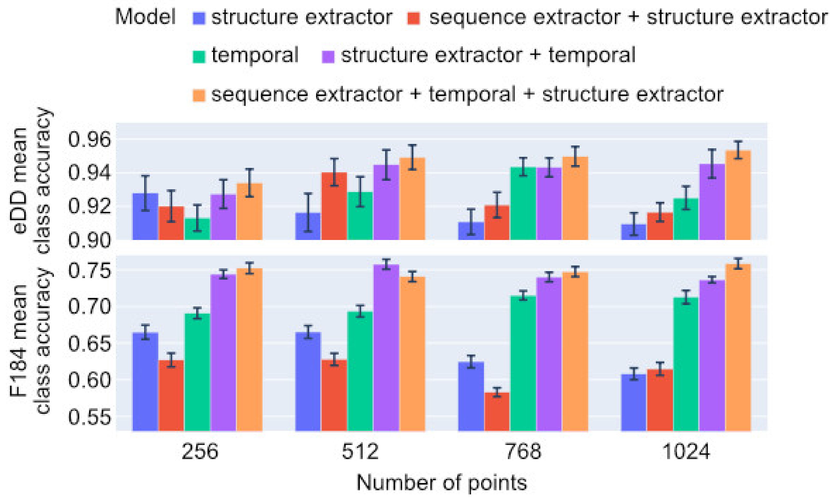
2.1. Classification
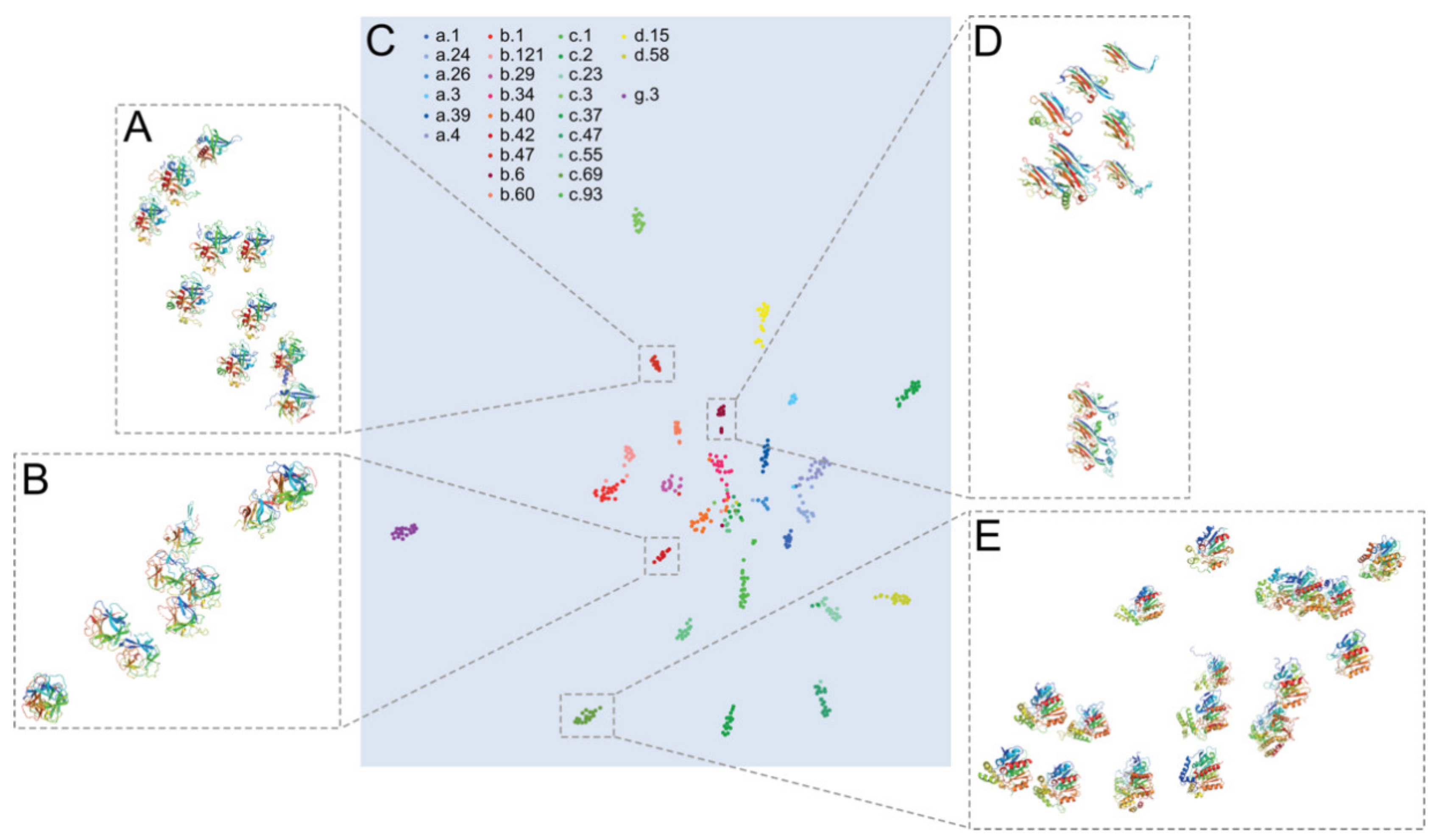
2.2. Embedding Protein Structures into ℝ2
3. Discussion
4. Materials and Methods
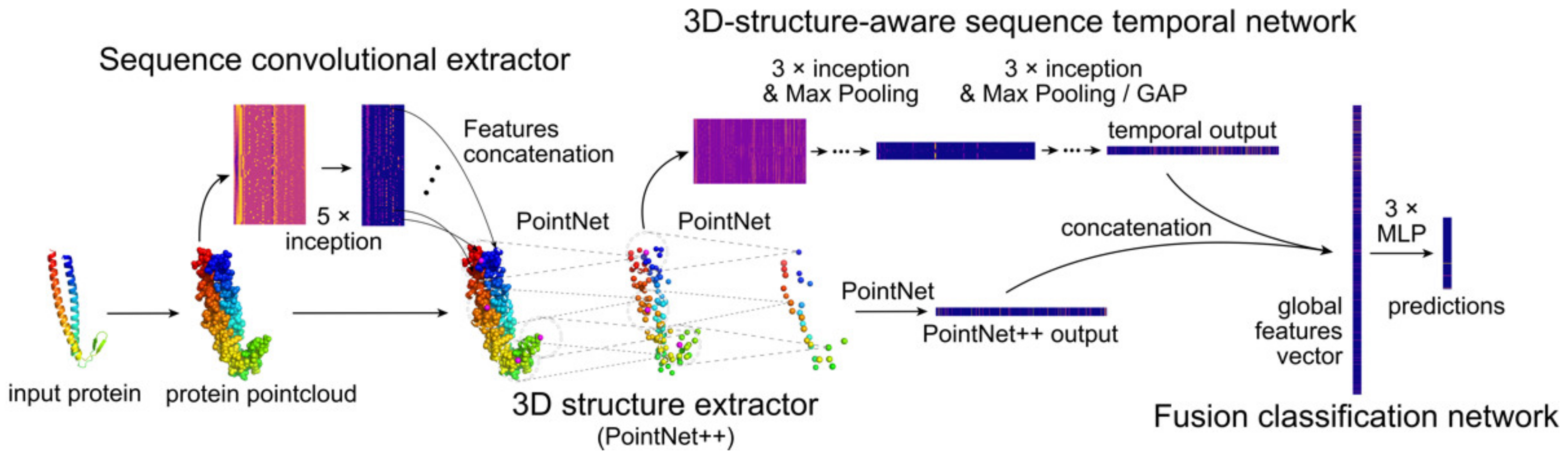
4.1. Architecture
- Sequence convolutional extractor;
- 3D structure extractor;
- 3D structure-aware sequence temporal network;
- Fusion and classification network.
4.1.1. Sequence Convolutional Extractor
4.1.2. 3D Structure Extractor
4.1.3. 3D structure-Aware Sequence Temporal Network
4.1.4. Fusion and Classification Network
4.1.5. Information Flow
4.2. Datasetes
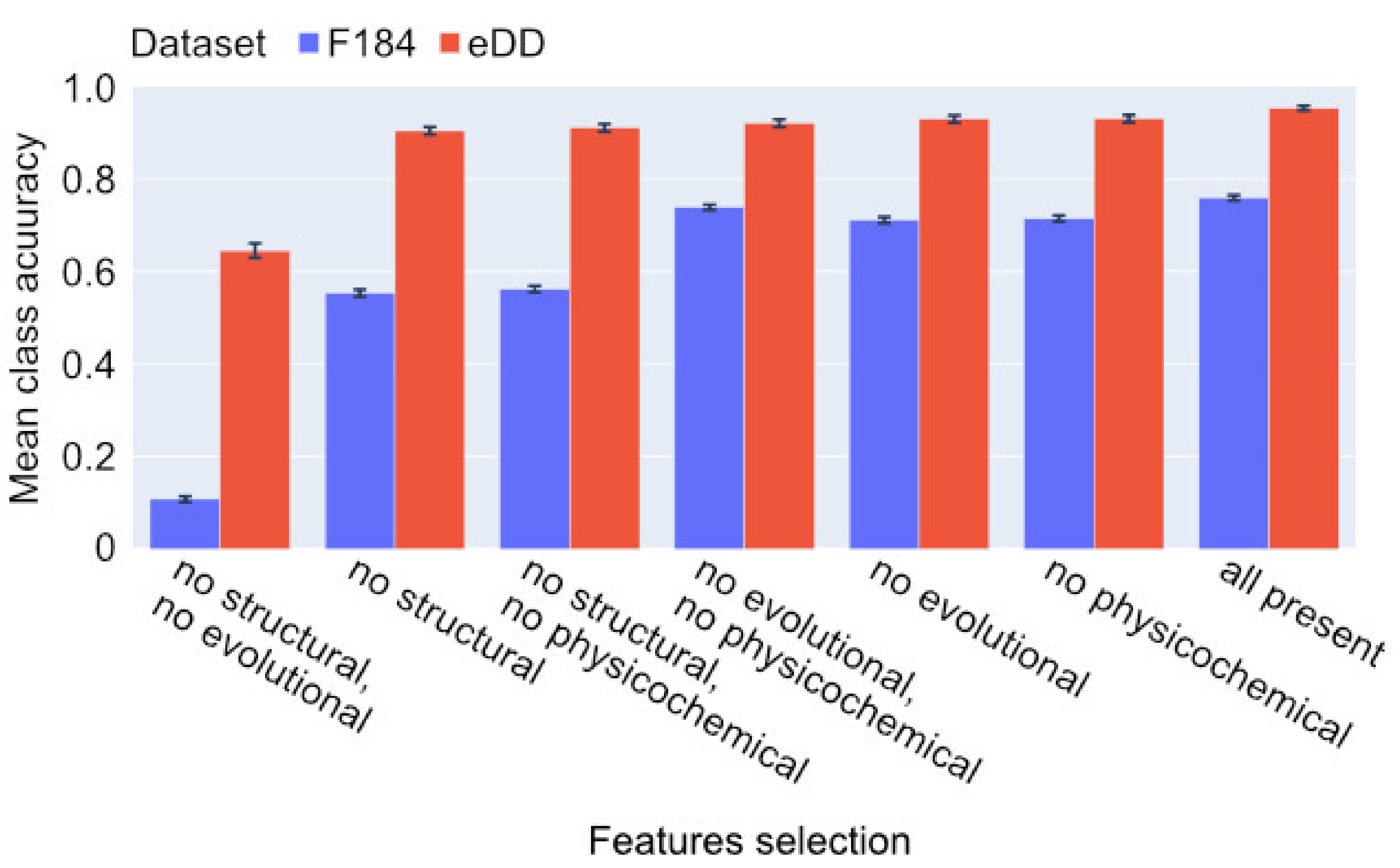
4.3. Features
4.4. Calculation of Accuracy
4.5. Computational Resources
5. Conclusions
Supplementary Materials
Author Contributions
Funding
Institutional Review Board Statement
Informed Consent Statement
Data Availability Statement
Acknowledgments
Conflicts of Interest
References
- Nakane, T.; Kotecha, A.; Sente, A.; McMullan, G.; Masiulis, S.; Brown, P.M.G.E.; Grigoras, I.T.; Malinauskaite, L.; Malinauskas, T.; Miehling, J.; et al. Single-particle cryo-EM at atomic resolution. Nature 2020, 587, 152–156. [Google Scholar] [CrossRef] [PubMed]
- Yip, K.M.; Fischer, N.; Paknia, E.; Chari, A.; Stark, H. Atomic-resolution protein structure determination by cryo-EM. Nature 2020, 587, 157–161. [Google Scholar] [CrossRef] [PubMed]
- wwPDB consortium. Protein Data Bank: The single global archive for 3D macromolecular structure data. Nucleic Acids Res. 2018, 47, D520–D528. [Google Scholar] [CrossRef] [Green Version]
- Guo, Y.; Wang, H.; Hu, Q.; Liu, H.; Liu, L.; Bennamoun, M. Deep learning for 3D point clouds: A survey. IEEE Trans. Pattern Anal. Mach. Intell. 2021, 43, 4338–4364. [Google Scholar] [CrossRef]
- Qi, C.R.; Su, H.; Mo, K.; Guibas, L.J. Pointnet: Deep learning on point sets for 3D classification and segmentation. In Proceedings of the IEEE Conference on Computer Vision and Pattern Recognition, Honolulu, HI, USA, 21–26 July 2017; pp. 652–660. [Google Scholar]
- DeFever, R.S.; Targonski, C.; Hall, S.W.; Smith, M.C.; Sarupria, S. A generalized deep learning approach for local structure identification in molecular simulations. Chem. Sci. 2019, 10, 7503–7515. [Google Scholar] [CrossRef] [PubMed] [Green Version]
- Benhabiles, H.; Hammoudi, K.; Windal, W.; Melkemi, M.; Cabani, A. A transfer learning exploited for indexing protein structures from 3D point clouds. In Processing and Analysis of Biomedical Information; Lepore, N., Brieva, J., Romero, E., Racoceanu, D., Joskowicz, L., Eds.; Springer International Publishing: Cham, Switzerland, 2018; pp. 82–89. [Google Scholar]
- Toomer, D. Predicting Protein Functional Sites through Deep Graph Convolutional Neural Networks on Atomic Point-Clouds. 2020. Available online: http://cs230.stanford.edu/projects_winter_2020/reports/32610279.pdf (accessed on 23 February 2022).
- Nguyen, T.; Le, H.; Quinn, T.P.; Nguyen, T.; Le, T.C.; Venkatesh, S. GraphDTA: Predicting drug–target binding affinity with graph neural networks. Bioinformatics 2021, 37, 1140–1147. [Google Scholar] [CrossRef] [PubMed]
- Qi, C.R.; Yi, L.; Su, H.; Guibas, L.J. Pointnet++: Deep hierarchical feature learning on point sets in a metric space. In Proceedings of the Advances in Neural Information Processing Systems 30 (NIPS 2017), Long Beach, CA, USA, 4–9 December 2017; pp. 5099–5108. [Google Scholar]
- Dubchak, I.; Muchnik, I.; Holbrook, S.R.; Kim, S.H. Prediction of protein folding class using global description of amino acid sequence. Proc. Natl. Acad. Sci. USA 1995, 92, 8700–8704. [Google Scholar] [CrossRef] [Green Version]
- Cheng, J.; Baldi, P. A machine learning information retrieval approach to protein fold recognition. Bioinformatics 2006, 22, 1456–1463. [Google Scholar] [CrossRef] [Green Version]
- Hou, J.; Adhikari, B.; Cheng, J. DeepSF: Deep convolutional neural network for mapping protein sequences to folds. Bioinformatics 2018, 34, 1295–1303. [Google Scholar] [CrossRef]
- Xia, J.; Peng, Z.; Qi, D.; Mu, H.; Yang, J. An ensemble approach to protein fold classification by integration of template-based assignment and support vector machine classifier. Bioinformatics 2017, 33, 863–870. [Google Scholar] [CrossRef]
- Sudha, P.; Ramyachitra, D.; Manikandan, P. Enhanced artificial neural network for protein fold recognition and structural class prediction. Gene Rep. 2018, 12, 261–275. [Google Scholar] [CrossRef]
- Liu, B.; Zhu, Y.; Yan, K. Fold-LTR-TCP: Protein fold recognition based on triadic closure principle. Brief. Bioinf. 2019, 21, 2185–2193. [Google Scholar] [CrossRef]
- Maaten, L.v.d.; Hinton, G. Visualizing data using t-sne. J. Mach. Learn. Res. 2008, 9, 2579–2605. [Google Scholar]
- Schrödinger, LLC. The PyMOL Molecular Graphics System, Version 1.8. 2015. Available online: https://pymol.org/2/ (accessed on 14 January 2022).
- Fox, N.K.; Brenner, S.E.; Chandonia, J.M. SCOPe: Structural classification of proteins—Extended, integrating SCOP and ASTRAL data and classification of new structures. Nucleic Acids Res. 2014, 42, D304–D309. [Google Scholar] [CrossRef] [PubMed]
- Jin, X.; Awale, M.; Zasso, M.; Kostro, D.; Patiny, L.; Reymond, J.L. PDB-Explorer: A web-based interactive map of the protein data bank in shape space. BMC Bioinform. 2015, 16, 339. [Google Scholar] [CrossRef] [Green Version]
- Li, Z.; Yan, X.; Wei, Q.; Gao, X.; Wang, S.; Cui, S. Pointsite: A Point Cloud Segmentation Tool for Identification of Protein Ligand Binding Atoms. 2019. Available online: https://www.biorxiv.org/content/10.1101/831131v1.full (accessed on 14 January 2022).
- Altschul, S.F.; Gish, W.; Miller, W.; Myers, E.W.; Lipman, D.J. Basic local alignment search tool. J. Mol. Biol. 1990, 215, 403–410. [Google Scholar] [CrossRef]
- Wei, L.Y.; Liao, M.H.; Gao, X.; Zou, Q. Enhanced protein fold prediction method through a novel feature extraction technique. IEEE Trans. Nanobiosci. 2015, 14, 649–659. [Google Scholar] [CrossRef]
- Chen, D.Z.; Tian, X.Y.; Zhou, B.; Gao, J. Profold: Protein fold classification with additional structural features and a novel ensemble classifier. BioMed. Res. Int. 2016, 2016, 6802832. [Google Scholar] [CrossRef] [Green Version]
- Lyons, J.; Paliwal, K.K.; Dehzangi, A.; Hefferman, R.; Tsunoda, T.; Sharma, A. Protein fold recognition using HMM–HMM alignment and dynamic programming. J. Theor. Biol. 2016, 393, 67–74. [Google Scholar] [CrossRef]
- Yan, K.; Fang, X.Z.; Xu, Y.; Liu, B. Protein fold recognition based on multi-view modeling. Bioinformatics 2019, 35, 2982–2990. [Google Scholar] [CrossRef]
- Refahi, M.S.; Mir, A.; Nasiri, J.A. A novel fusion based on the evolutionary features for protein fold recognition using support vector machines. Sci. Rep. 2020, 10, 14368. [Google Scholar] [CrossRef] [PubMed]
- Qin, X.; Liu, M.; Zhang, L.; Liu, G. Structural protein fold recognition based on secondary structure and evolutionary information using machine learning algorithms. Comput. Biol. Chem. 2021, 91, 107456. [Google Scholar] [CrossRef] [PubMed]
- Holm, L. DALI and the persistence of protein shape. Prot. Sci. 2020, 29, 128–140. [Google Scholar] [CrossRef] [PubMed] [Green Version]
- Holm, L. Benchmarking fold detection by DaliLite v.5. Bioinformatics 2019, 35, 5326–5327. [Google Scholar] [CrossRef] [PubMed]
- Van Kempen, M.; Kim, S.S.; Tumescheit, C.; Mirdita, M.; Söding, J.; Steinegger, M. Foldseek: Fast and Accurate Protein Structure Search. 2022. Available online: https://www.biorxiv.org/content/10.1101/2022.02.07.479398v1.full (accessed on 23 February 2022).
- Agrawal, V.; Kishan, R.K. Functional evolution of two subtly different (similar) folds. BMC Struct. Biol. 2001, 1, 5. [Google Scholar] [CrossRef]
- Mura, C.; Veretnik, S.; Bourne, P.E. The Urfold: Structural similarity just above the superfold level? Protein Sci. 2019, 28, 2119–2126. [Google Scholar] [CrossRef] [Green Version]
- Youkharibache, P.; Veretnik, S.; Li, Q.; Stanek, K.A.; Mura, C.; Bourne, P.E. The Small β-Barrel Domain: A Survey-Based Structural Analysis. Structure 2019, 27, 6–26. [Google Scholar] [CrossRef] [Green Version]
- Sadowski, M.I.; Taylor, W.R. On the evolutionary origins of “Fold Space Continuity”: A study of topological convergence and divergence in mixed alpha-beta domains. J. Struct. Biol. 2010, 172, 244–252. [Google Scholar] [CrossRef]
- Westhead, D.R.; Slidel, T.W.; Flores, T.P.; Thornton, J.M. Protein structural topology: Automated analysis and diagrammatic representation. Prot. Sci. 1999, 8, 897–904. [Google Scholar] [CrossRef] [Green Version]
- Zhang, D.; Iyer, L.M.; Burroughs, A.M.; Aravind, L. Resilience of biochemical activity in protein domains in the face of structural divergence. Curr. Opin. Struct. Biol. 2014, 26, 92–103. [Google Scholar] [CrossRef] [Green Version]
- Petrey, D.; Honig, B. Is protein classification necessary? Toward alternative approaches to function annotation. Curr. Opin. Struct. Biol. 2009, 19, 363–368. [Google Scholar] [CrossRef] [PubMed] [Green Version]
- Fontove, F.; Del Rio, G. Residue Cluster Classes: A unified protein representation for efficient structural and functional classification. Entropy 2020, 22, 472. [Google Scholar] [CrossRef] [PubMed] [Green Version]
- Pombo, A.; Dillon, N. Three-dimensional genome architecture: Players and mechanisms. Nat. Rev. Mol. Cell Biol. 2015, 16, 245–257. [Google Scholar] [CrossRef] [PubMed]
- Jowhar, Z.; Gudla, P.R.; Shachar, S.; Wangsa, D.; Russ, J.L.; Pegoraro, G.; Ried, T.; Raznahan, A.; Misteli, T. HiCTMap: Detection and analysis of chromosome territory structure and position by high-throughput imaging. Methods 2018, 142, 30–38. [Google Scholar] [CrossRef]
- Marella, N.V.; Bhattacharya, S.; Mukherjee, L.; Xu, J.; Berezney, R. Cell type specific chromosome territory organization in the interphase nucleus of normal and cancer cells. J. Cell Physiol. 2009, 221, 130–138. [Google Scholar] [CrossRef]
- Szegedy, C.; Liu, W.; Jia, Y.; Sermanet, P.; Reed, S.; Anguelov, D.; Erhan, D.; Vanhoucke, V.; Rabinovich, A. Going deeper with convolutions. In Proceedings of the IEEE Conference on Computer Vision and Pattern Recognition, Boston, MA, USA, 7–12 June 2015; pp. 1–9. [Google Scholar]
- Yang, J.; Wang, Y.; Zhang, Y. ResQ: An Approach to Unified Estimation of B-Factor and Residue-Specific Error in Protein Structure Prediction. J. Mol. Biol. 2016, 428, 693–701. [Google Scholar] [CrossRef] [PubMed] [Green Version]
- Bramer, D.; Wei, G.W. Blind prediction of protein B-factor and flexibility. J. Chem. Phys. 2018, 149, 134107. [Google Scholar] [CrossRef]
- Yang, J.Y.; Chen, X. Improving taxonomy-based protein fold recognition by using global and local features. Proteins 2011, 79, 2053–2064. [Google Scholar] [CrossRef]
- Sacquin-Mora, S. Fold and flexibility: What can proteins’ mechanical properties tell us about their folding nucleus? J. R. Soc. Interface 2015, 12, 20150876. [Google Scholar] [CrossRef]
- Kabsch, W.; Sander, C. Dictionary of protein secondary structure: Pattern recognition of hydrogen-bonded and geometrical features. Biopolymers 1983, 22, 2577–2637. [Google Scholar] [CrossRef]
- Dehzangi, A.; Sharma, A.; Lyons, J.; Paliwal, K.K.; Sattar, A. A mixture of physicochemical and evolutionary-based feature extraction approaches for protein fold recognition. Int. J. Data Min. Bioinform. 2015, 11, 115–138. [Google Scholar] [CrossRef] [PubMed] [Green Version]
- Grantham, R. Amino acid difference formula to help explain protein evolution. Science 1974, 185, 862–864. [Google Scholar] [CrossRef] [PubMed]
- Charton, M.; Charton, B.I. The structural dependence of amino acid hydrophobicity parameters. J. Theor. Biol. 1982, 99, 629–644. [Google Scholar] [CrossRef]
- Casari, G.; Sippl, M.J. Structure-derived hydrophobic potential. Hydrophobic potential derived from X-ray structures of globular proteins is able to identify native folds. J. Mol. Biol. 1992, 224, 725–732. [Google Scholar] [CrossRef]
- Altschul, S.F.; Madden, T.L.; Schäffer, A.A.; Zhang, J.; Zhang, Z.; Miller, W.; Lipman, D.J. Gapped BLAST and PSI-BLAST: A new generation of protein database search programs. Nucleic Acids Res. 1997, 25, 3389–3402. [Google Scholar] [CrossRef] [PubMed] [Green Version]
- Kingma, D.P.; Ba, J. Adam: A Method for Stochastic Optimization. 2019. Available online: https://arxiv.org/abs/1412.6980 (accessed on 14 January 2022).
- Stepniewska-Dziubinska, M.M.; Zielenkiewicz, P.; Siedlecki, P. Improving detection of protein-ligand binding sites with 3D segmentation. Sci. Rep. 2020, 10, 5035. [Google Scholar] [CrossRef] [PubMed] [Green Version]


| Dataset | |||
|---|---|---|---|
| BioS2Net without: | eDD | F184 | Both |
| Sequence convolutional extractor | −0.65% | −0.52% | −0.58% |
| 3D structure extractor | −1.91% | −4.68% | −3.29% |
| 3D structure-aware sequence temporal network | −2.22% | −13.66% | −7.94% |
| Method | Accuracy | References |
|---|---|---|
| PFPA (2015) | 92.6% | [23] |
| ProFold (2016) | 93.2% | [24] |
| PHMM-DP (2016) | 92.9% | [25] |
| Xia et al. (2017) | 94.5% | [14] |
| MV-fold (2019) | 94.8% | [26] |
| MT-fold (2019) | 97.1% | [26] |
| Refahi et al. (2020) | 91.2% | [27] |
| Qin et al. (2021) | 93.5% | [28] |
| BioS2Net | 95.4% | This work |
| Index | Feature | Value | Feature Type | Feature Level |
|---|---|---|---|---|
| 1 | x | ℝ | Coordinate | Atomic |
| 2 | y | ℝ | ||
| 3 | z | ℝ | ||
| 4 | B factor | [0, 1] | Structural | |
| 5 | Occupancy | [0, 1] | ||
| 6 | Distance from N-terminus | [0, 1] | ||
| 7 | Is ⍺-helix | Boolean | Amino acids | |
| 8 | Is β-sheet | Boolean | ||
| 9 | Accessible area | [0, 1] | ||
| 10–29 | Amino acid | Boolean | ||
| 30 | Charge | [−1, 1] | Physicochemical | |
| 31 | Polarity | [0, 1] | ||
| 32 | Polarizability | [0, 1] | ||
| 33 | Hydrophobicity | [0, 1] | ||
| 34–53 | PSSM | [0, 1] | Evolutionary |
Publisher’s Note: MDPI stays neutral with regard to jurisdictional claims in published maps and institutional affiliations. |
© 2022 by the authors. Licensee MDPI, Basel, Switzerland. This article is an open access article distributed under the terms and conditions of the Creative Commons Attribution (CC BY) license (https://creativecommons.org/licenses/by/4.0/).
Share and Cite
Roethel, A.; Biliński, P.; Ishikawa, T. BioS2Net: Holistic Structural and Sequential Analysis of Biomolecules Using a Deep Neural Network. Int. J. Mol. Sci. 2022, 23, 2966. https://doi.org/10.3390/ijms23062966
Roethel A, Biliński P, Ishikawa T. BioS2Net: Holistic Structural and Sequential Analysis of Biomolecules Using a Deep Neural Network. International Journal of Molecular Sciences. 2022; 23(6):2966. https://doi.org/10.3390/ijms23062966
Chicago/Turabian StyleRoethel, Albert, Piotr Biliński, and Takao Ishikawa. 2022. "BioS2Net: Holistic Structural and Sequential Analysis of Biomolecules Using a Deep Neural Network" International Journal of Molecular Sciences 23, no. 6: 2966. https://doi.org/10.3390/ijms23062966