Abstract
To ensure efficiency in discovery and development, the application of computational technology is essential. Although virtual screening techniques are widely applied in the early stages of drug discovery research, the computational methods used in lead optimization to improve activity and reduce the toxicity of compounds are still evolving. In this study, we propose a method to construct the residue interaction profile of the chemical structure used in the lead optimization by performing “inverse” mixed-solvent molecular dynamics (MSMD) simulation. Contrary to constructing a protein-based, atom interaction profile, we constructed a probe-based, protein residue interaction profile using MSMD trajectories. It provides us the profile of the preferred protein environments of probes without co-crystallized structures. We assessed the method using three probes: benzamidine, catechol, and benzene. As a result, the residue interaction profile of each probe obtained by MSMD was a reasonable physicochemical description of the general non-covalent interaction. Moreover, comparison with the X-ray structure containing each probe as a ligand shows that the map of the interaction profile matches the arrangement of amino acid residues in the X-ray structure.
1. Introduction
Drug development is a cost-intensive and time-consuming process. The cost is estimated to be more than USD two billion, and it may take 10–15 years for a new drug to reach the market [1]. To reduce costs, computational techniques have been applied in various drug development studies, and many studies have successfully discovered new therapeutic compounds using these techniques [2,3,4,5,6,7,8,9,10]. In the early stages of drug discovery, virtual screening (VS) techniques such as docking simulations are frequently used to discover seed compounds [11,12,13]. Kelly et al. showed that high-throughput virtual screening (HTVS) produced more than 10-fold hit rates compared to traditional HTS [14]. Computational methods for lead optimization to improve the activity of compounds are also proposed, such as MP-CAFEE [15], free energy perturbation (FEP) [16,17], and quantum mechanical (QM) methods [18]. These methods focused on the binding affinity estimation of given candidate compounds with considerable computational cost; however, methods guiding or proposing the next substituent of hit compounds in the lead optimization phase are still evolving.
To improve activity and selectivity, structural optimization that is strongly and specifically directed at the target protein is necessary. Therefore, the mechanism by which proteins recognize compounds and the prediction of protein–ligand binding modes are important in lead optimization. Several studies have been reported that comprehensively analyze interaction patterns from protein–ligand complex structures registered in the Protein Data Bank (PDB) [19]. Imai et al. focused on 14 polar and aromatic amino acid side chains and carried out contact analysis for protein–ligand complex crystal structures in the PDB [20]. Wang et al. generated 4032 fragments from 71,798 ligands and obtained fragment–residue interaction profiles [21]. Furthermore, Kasahara et al. reported that 63.4% of the ligand atoms exhibited one or more interaction patterns, 25.7% of the ligand atoms interacted without patterns, and the rest had no direct interaction [22]. However, these interaction patterns have been analyzed only from known databases, and the analysis is limited to the well-experimented functional groups. In addition, the interaction patterns of the functional groups investigated in these studies were studied while binding to the target as part of the compound, and the environment of the protein to which functional group fragments match has not been directly investigated.
Mixed-solvent molecular dynamics (MSMD) simulations involve MD in the presence of explicit water molecules mixed with probe molecules or functional group fragments such as for hotspot detection [23,24] and binding site identification [25,26]. MSMD considers the flexibility of proteins and can discover hotspots where probes can bind. These hotspots indicate the protein environment preferred by specific probes. Thus, by analyzing the interaction pattern between the probe and the protein environment sampled by MSMD, it is possible to analyze the binding ability and interaction pattern of individual probes, not part of the functional group of compounds. In particular, by applying drug-like probes with few reported crystal structures to MSMD, the environment of the protein binding site to which the unique probe binds can be sampled.
In this article, we propose an “inverse” MSMD for analyzing a probe’s preference of interaction patterns. First, MSMD simulations with 15 diverse proteins were performed to sample various protein residue environments preferred by the probe. The residue environments were then integrated to a residue interaction profile, followed by the visualization of it. We assessed the proposed analysis using three probes with an aromatic ring: benzamidine, catechol, and benzene. Their residue interaction profiles provided a physicochemical account of general non-covalent interactions, such as electrostatic interactions, hydrogen bonding interactions, and amide- stacking interactions. Moreover, the profiles were consistent with the experimental co-crystalized structures, which supports the ability of the proposed method to detect the actual interaction patterns of functional groups. This is the first proposal and demonstration of the use of inverse MSMD.
2. Materials and Methods
2.1. Preparation of Proteins
The selection of proteins used in MSMD sampling is crucial to obtain the various residue environments utilized to construct a residue interaction profile. We chose 15 proteins that were previously selected by Soga et al. [27] because they collected the proteins considering their diversity. A list of proteins is shown in Table 1. All proteins were pre-processed using the following procedure: Protein Preparation Wizard and Prime [28] in Schrodinger suite 2020-3 (Schrodinger, Inc., New York, NY, USA) were used to fill the missing loops, side chains, and atoms for all of the selected proteins. N- and C-termini were capped using N-methyl amide (NME) and acetyl (ACE) capping groups, respectively. Subsequently, the ligands, co-factors, and additive molecules were removed. Hydrogens were placed with consideration of hydrogen bonding and ionization states of pH = 7 with PROPKA [29]. Water molecules with less than two hydrogen bonds to a protein in the crystal structures were removed, followed by structure optimization with the OPLS3e force field. Note that the N-terminal of glycoside hydrolase (PDBID: 1H4G) and C-terminal of endo-1,4-β-xylanase A precursor (PDBID: 1E0X) were removed before the procedure because of non-standard amino acid and missing main chain atoms, respectively.

Table 1.
The list of proteins utilized in this and originally collected by Soga et al. [27].
2.2. Preparation of Probes
The probe of interest was then pre-processed. The restrained electrostatic potential (RESP) procedure in the Antechamber module of AmberTools18 [30] was employed to fit the partial charges to the electrostatic potential, which was calculated using Gaussian 16 Rev B.01 [31]. First, all probe structures were optimized at the B3LYP/6-31G(d) level. Then, the electrostatic potentials were calculated at the HF level using the optimized structures. The centers of the electrostatic potentials were placed at the center of each atom. Additional force field parameters for the probes were derived using the general AMBER force field 2 (GAFF2), unless otherwise stated.
2.3. Mixed-Solvent Molecular Dynamics (MSMD)
We conducted MSMD using the protocol of EXPRORER [32]. It is worth noting that the initial positions of the probes affect the results, especially in short MD simulations, and this initial position dependency influences the convergence of the results of the analysis. To achieve efficient sampling, the following protocol was independently performed 20 times with different initial probe coordinates. The procedure was divided into three steps, as described below.
2.3.1. Initial System Generation
The probes were randomly placed around the protein at a concentration of 0.25 M using PACKMOL 18.169 [33]. The high concentration enables effective sampling of residue environments. Second, the system was solvated with water using the LEaP module of AmberTools18. The Amber ff14SB force field and the TIP3P model [34] were used for the protein and water molecules, respectively. Additionally, a Lennard–Jones force field term with the parameters (ϵ = 10−6 kcal/mol; Rmin = 20 Å) was introduced only between the center of the probes to prevent their aggregation.
2.3.2. Minimization, Heating, and Equilibration
After the construction of the initial structures, the systems were minimized to include 200 steps using the steepest descent algorithm with harmonic position restraints on the heavy solute atoms (force constant, 10 kcal/mol/Å2), and then the systems were minimized a further 200 steps using the steepest descent algorithm without any position restraints. After minimization, the system was heated gradually to 300 K during 200 ps constant-NVT MD simulations with harmonic position restraints on the solute heavy atoms (force constant, 10 kcal/mol/Å2). During the subsequent 800 ps constant-NPT MD simulations at 300 K and 105 Pa, the force constants of the position restraints were gradually reduced to 0 kcal/mol/Å2. The P-LINCS algorithm [35] was used to constrain all bond lengths involving hydrogen atoms, which allowed the use of 2 fs time steps. Temperature and pressure were controlled using a stochastic velocity-rescaling (V-rescale) algorithm [36,37,38] and a Berendsen barostat [39], respectively. Simulations were performed using GROMACS 2019.4 [40]. The ParmEd module [41] was used to convert the AMBER parameter/topology file format to that used by GROMACS.
2.3.3. Production Run
After equilibration, 40 ns constant-NPT MD simulations at 300 K and 105 Pa without position restraints were performed. All settings were the same as the initial equilibration step, but a Parrinello–Rahman barostat [42] was used instead of a Berendsen barostat. Snapshots were taken every 10 ps in the 20–40 ns; thus, 2000 snapshots were produced per MSMD simulation.
2.4. Inverse MSMD: Construction of Residue Interaction Profile
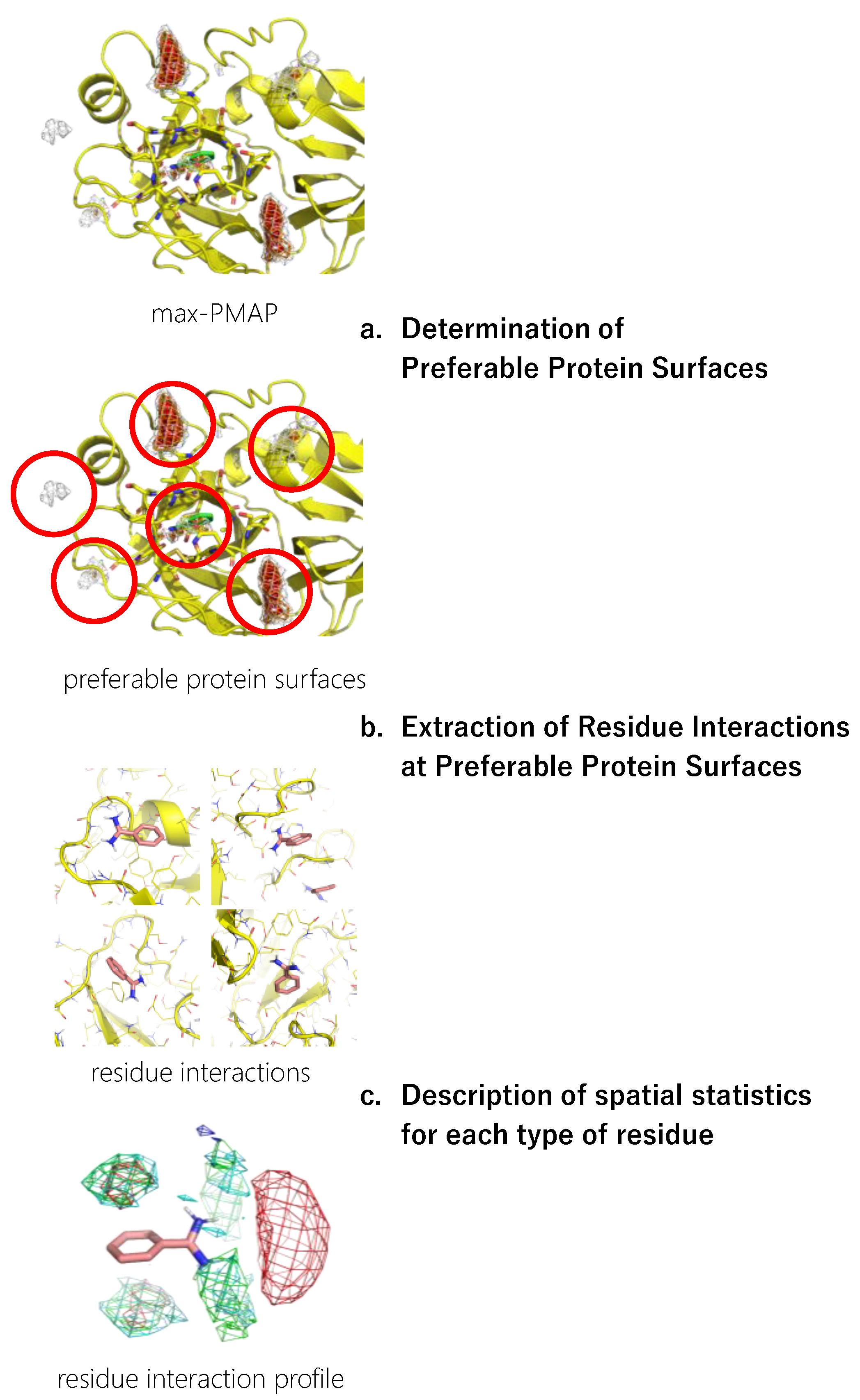
The workflow for constructing a residue interaction profile from the MSMD simulation is shown in Figure 1. The detailed procedure is described in this section.

Figure 1.
A workflow of inverse MSMD to construct a residue interaction profile.
2.4.1. Determination of Preferable Protein Surfaces
The concentration of probes in the MSMD simulation was unrealistically high, which could cause artificial interaction profiles even though the concentration is sometimes used in other MSMD protocols [43]. To omit such artifacts, we limited the residue environment sampling based on the binding preference of the probes. First, the spatial probability distribution map (PMAP) was calculated using the following procedure: Atoms in the snapshots were binned into 1 Å × 1 Å × 1 Å grid voxels, and the voxel occupancy of probe heavy atoms was calculated. To focus on the protein surface, was a set of voxels within 5 Å from the protein atoms, and the values at voxel were discarded. Then, the values were scaled such that the summation of voxels in was 1.0.
Probes were placed uniformly among the system, resulting in the underestimation of the probability at deep pockets where access is difficult. Thus, to reduce the underestimation, the largest value among the 20 PMAPs generated from each independent trajectory was stored for each voxel in in the second step. The product was named max-PMAP. Even for a deep pocket where a probe will bind strongly but will rarely approach, a considerable value of voxel of max-PMAP was observed if the binding occurred only at least once. Note that the summation of voxels of max-PMAP was greater than 1.0, while it originated from the probability. Finally, we defined a preferable protein surface of a probe as voxels with max-PMAP values equal to or greater than 0.2, which is determined by visual inspection. Note that the preferable protein surface includes surfaces exposed to solvent as well as deeper binding pockets (Figure 2). The regions indicate the protein surfaces where the probe stably exists.
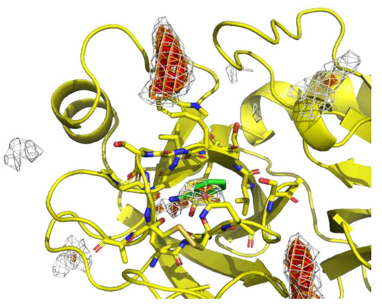
Figure 2.
An example of preferable protein surfaces based-on max-PMAP. Positions shown as meshes are preferable protein surfaces, where the value of max-PMAP is higher than a threshold. The gray, orange, and red meshes show the same max-PMAP but different thresholds.
2.4.2. Extraction of Residue Environments at Preferable Protein Surfaces
Next, the protein residue environments around the probe molecules were extracted. As previously mentioned, we sampled poses on the preferable protein surfaces of the probe. Extraction of preferable protein surfaces of a probe was performed for each snapshot, and the probe and amino acid residues around the probe were extracted after detecting the probe on preferable protein surfaces. Here, we defined “amino acid residues around the probe” as protein residues with at least one heavy atom that is within 4 Å from any heavy atom of the probe molecule (Figure 3).
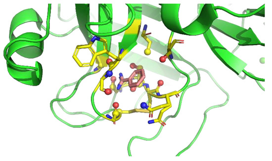
Figure 3.
Definition of amino acid residues around the probe. Yellow residues are “amino acid residues around the probe”. Amino acid heavy atoms within 4 Å from any heavy atom of the probe molecule (red molecule) are shown as balls.
2.4.3. Description of Spatial Statistics for Each Type of Residue
Finally, a residue interaction profile, or a set of spatial distribution of residues around a probe, was described with the following steps. All the sampled residue environments were aligned by referring to the designated atoms of the probe molecule. The Cβ atoms of each type of residue were spatially binned into 1 Å × 1 Å × 1 Å grid voxels. The types of residues used in this study are listed in Table 2. Note that we used Cβ atoms rather than the side chain atoms (e.g., nitrogen atoms of Lys and aromatic carbon atoms of Phe) because our aim was to analyze the protein environment, and the direction of the tip of the side chains is easily changed.
Table 2.
Types of residues used in this study. Note that glycine is not included in this table, since it does not have any Cβ atoms.
2.5. Implementation
The scripts used to generate a residue interaction profile of a probe were implemented using Python with Biopython [44]. The implementation is included in a GitHub repository EXPRORER_MSMD https://github.com/keisuke-yanagisawa/exprorer_msmd (accessed on 22 April 2022) under the MIT license.
3. Results
We tested the proposed method with benzamidine, catechol, and benzene. Ring systems are key scaffold components in medicinal chemistry [45]; therefore, we selected these probes with a ring system as examples of available probes. Note that since the GAFF2 force field incorrectly parameterized the amidino group of benzamidine, we manually assigned “nc” and “cc” GAFF2 atom types for nitrogen and carbon atoms of the amidino group, respectively, to maintain planarity of the functional group. Additionally, structural alignment of the probes was performed with all carbon atoms for benzamidine and with all heavy atoms for catechol and benzene.
3.1. Benzamidine: Evaluation of the Method
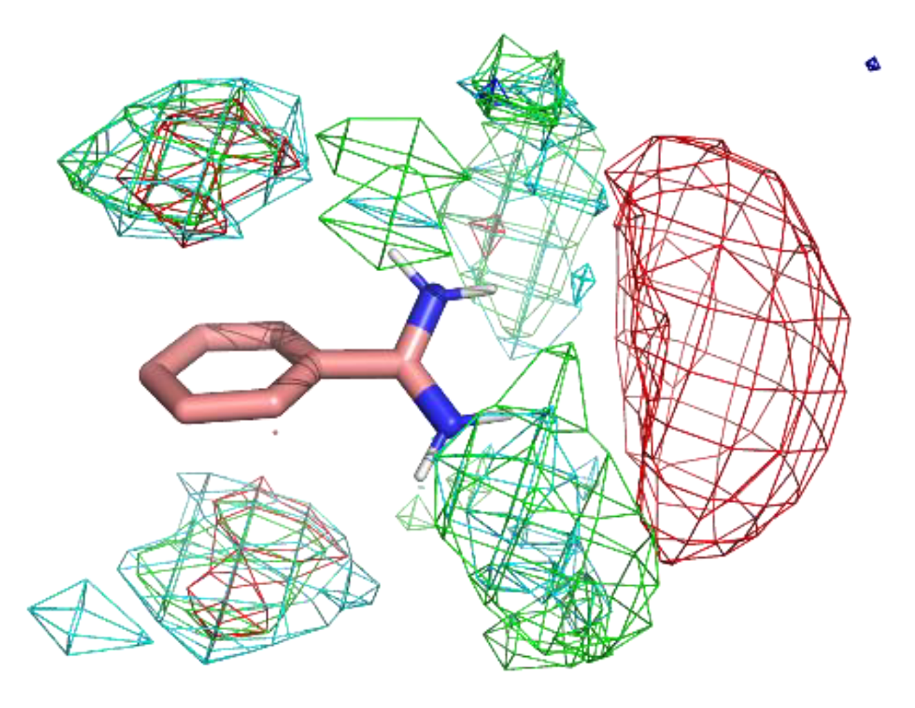
Figure 4 shows the residue interaction profile of benzamidine. Benzamidine has a basic group and the residue interaction profile correctly and clearly depicted the position of acidic residues. Furthermore, profiles of multiple types of residues were detected among the amidino group, indicating hydrogen bonds between the main chains and the amidino group (Figure 5). For the phenyl group, profiles of acidic, hydrophilic, and hydrophobic residues were detected in the vertical direction of the phenyl group. This suggests that the protocol captured amide- stacking [46]. Therefore, these profiles can provide a physicochemical account of general non-covalent interactions, and the results demonstrate the validity of the proposed method.

Figure 4.
The residue interaction profile of benzamidine. Green, cyan, gray, blue, and red meshes indicate profiles of hydrophobic, hydrophilic, aromatic, basic, and acidic residues, respectively. The molecule structure is that of benzamidine.
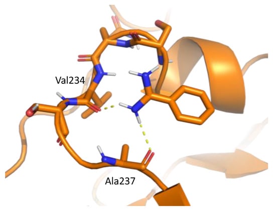
Figure 5.
An example of interaction pattern between benzamidine and penicillopepsin (PDBID: 2WEA) obtained from MSMD simulation. Yellow hashed lines show hydrogen bonds.
3.2. Catechol: Interaction Analysis of Hydroxy Groups
Catechol exists as a substructure in several ligands, such as dopamine. It has two hydroxy groups and a phenyl group. Although it does not have any net charge, which is different from benzamidine, hydroxy groups can form hydrogen bonds, resulting in stable binding to proteins.
The residue interaction profile of catechol is shown in Figure 6. Interestingly, the acidic group showed clear localization compared to the other residue groups. This indicates the possibility of detecting not only obvious interactions but also non-intuitive interactions. Further analysis regarding the same is provided in the discussion section. Additionally, the profiles of the phenyl group were similar to those of benzamidine; however, the areas of localization were wider than those of benzamidine. Ghanakota et al. showed that the wider localization of probe atoms can be converted to entropic terms [47]. Thus, the present observations may indicate weaker binding of a catechol substructure to proteins.
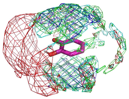
Figure 6.
The residue interaction profile of catechol. Green, cyan, gray, blue, and red meshes indicate profiles of hydrophobic, hydrophilic, aromatic, basic, and acidic residues, respectively. The molecule structure is that of catechol.
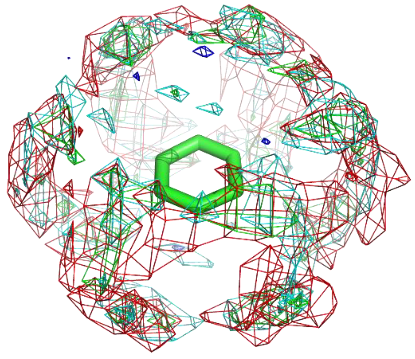
3.3. Benzene: Interaction Analysis of Phenyl Group Itself
Benzamidine and catechol both have phenyl groups, and their groups show clear residue interaction profiles. On the other hand, benzene did not display a profile in the vertical direction (Figure 7). Instead, weak profiles were detected in the horizontal direction. This indicates that interaction with only a single amide- stacking is insufficiently stable at the surface of proteins.
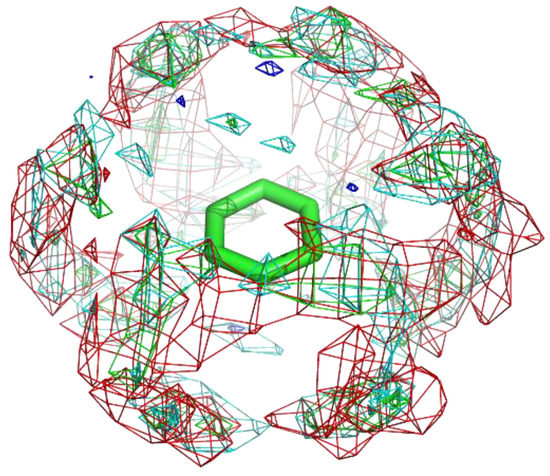
Figure 7.
The residue interaction profile of catechol. Green, cyan, gray, blue, and red meshes indicate profiles of hydrophobic, hydrophilic, aromatic, basic, and acidic residues, respectively. The molecule structure is that of catechol.
4. Discussion
4.1. Comparison to Co-Crystallized Structures
We compared the constructed residue interaction profiles and crystal structures for further verification of the appropriateness of the method.
4.1.1. Benzamidine
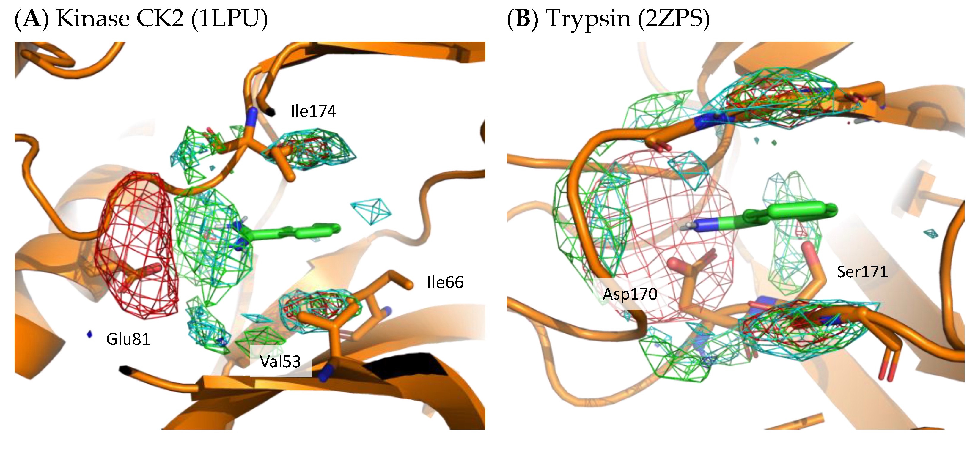
To demonstrate the validity of the residue interaction profile obtained by MSMD, the crystal structures of kinase CK2 (1LPU) and trypsin (2ZPS) with the residue interaction profile are shown in Figure 8. These crystal structures include benzamidine and can be compared to the preferred residue environment obtained by wet experiments. In the residue interaction profile of benzamidine obtained by MSMD, acidic residues are widely present near the amidino group. In kinase CK2 and trypsin, Glu81 and Asp170 are located near the profile of acidic residues. In kinase CK2, Val53, Ile66, and Ile174 are in the profile of hydrophobic residues above and below the aromatic ring of benzamidine. Notably, the profile of hydrophilic residues above and below the aromatic ring was suggested by MSMD. Ser171 of trypsin is located near the aromatic ring of benzamidine, which overlaps with the profile of hydrophilic residues. These two examples of X-ray structures, which are not included in the set of proteins for MSMD simulation, suggest that the residue interaction profile of a probe is reasonable and has generalization performance for any protein.

Figure 8.
X-ray structure with residue interaction profile of benzamidine obtained from MSMD simulation. (A) Kinase CK2 with benzamidine (PDBID: 1LPU); (B) trypsin with benzamidine (PDBID: 2ZPS). Green, cyan, gray, blue, and red meshes indicate profiles of hydrophobic, hydrophilic, aromatic, basic, and acidic residues, respectively.
4.1.2. Catechol
To validate the residue interaction profile of catechol obtained by MSMD, we compared it with X-ray structures that included catechol molecules. Figure 9 shows the X-ray structures of catalase and protocatechuate 3,4-dioxygenase, including catechol. On superimposing the residue interaction profile of catechol over the X-ray structure, Asp110 of catalase is in the profile of acidic residues. The hydrophobic residue interaction profile above and below the aromatic ring contains Leu150 and Leu181 of catalase and Leu35 of protocatechuate 3,4-dioxygenase. In addition, the crystal structure of protocatechuate 3,4-dioxygenase showed that Lys355 overlapped with the interaction profile of the basic residues. The amino acid residues around catechol in these X-ray structures are consistent with the residue interaction profile obtained by MSMD and support the simulation results. Again, these two proteins were not included in the set of proteins for MSMD simulation; thus, it indicates the generalization performance of the profile and the proposed method itself.
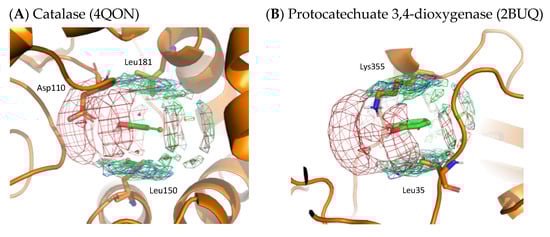
Figure 9.
X-ray structures with the residue interaction profile of catechol obtained from MSMD simulation. (A) Catalase with catechol (PDBID: 4QON); (B) protocatechuate 3,4-dioxygenase with catechol (PDBID: 2BUQ). Green, cyan, gray, blue, and red meshes indicate profiles of hydrophobic, hydrophilic, aromatic, basic, and acidic residues, respectively.
4.2. Detection of Aromatic Residues’ Profile
Despite several agreements between the X-ray structures and residue interaction profiles obtained from MSMD simulation, the profiles of aromatic residues were not detected sufficiently in spite of the threshold being the same among all residue types. One possible reason is the size of the side chains. Aromatic side chains have a relatively large structure compared to other types of residues, leading to a wider placement of the Cβ atoms. In this study, we aimed to show the residue-based interaction profile; thus, we focused on the Cβ atoms, which are common among almost all residues. However, it is also important to know the interaction profiles of specific atoms of side chains. The implementation already has the functionality to generate the profiles of any specific atoms, as well as Cβ. An exemplary interaction profile of aromatic rings is shown in Figure S1 in Supplementary Materials. Although it is a preliminary visualization and the signal of the profile is not stronger than that of Cβ atoms of acidic residues, the visualization result will suggest the - stacking more directly and will be informative for lead optimization.
4.3. Consideration of Binding Stability
In this study, we sampled residue environments at preferable protein surfaces to omit artifacts of MSMD simulation. The above results indicate that the sampled residue environments were informative; however, preferable protein surfaces can be classified into two types:
- Strong binding affinity between a probe molecule and the protein surface, which allows a single probe molecule to bind stably to the surface.
- Frequent access of probe molecules to the protein surface, which makes multiple probe molecules bind to the protein surface alternatively.
The aim of this sampling was to obtain a residue interaction profile in which a probe molecule binds stably. The protein surfaces of the first type were suitable for this purpose. The surfaces of the second type might be important in providing access to the binding site, but the binding affinity with the probe may not necessarily be strong.
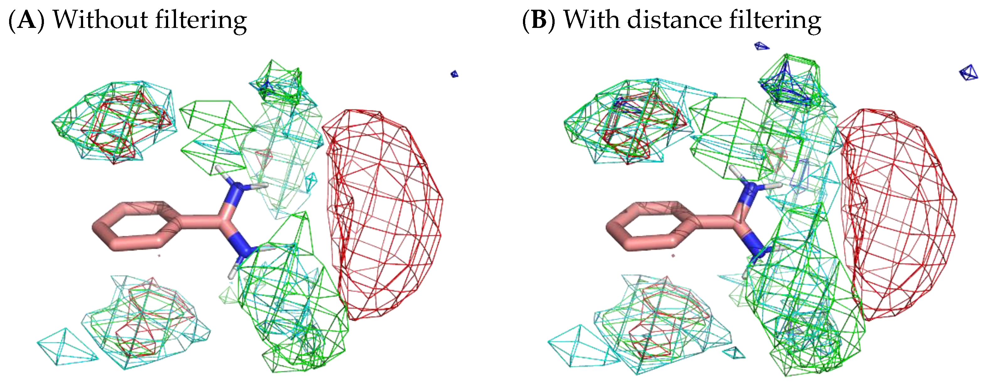
To obtain more appropriate residue interaction profiles, we tried to filter out residue environments whose probes were not stably situated. Here, we defined a stable probe molecule as a probe molecule that moved less than 3 Å from a place where the molecule was 500 ps before. The selection of stable samples omitted 77.4% of the residue environments of benzamidine, 88.0% of those of catechol, and 94.5% of those of benzene. However, Figure 10 reveals only a slight difference with and without filtering. Although filtering slightly enhanced the localization of residues, the results indicated that there was no significant difference between stable surfaces and accessible surfaces.
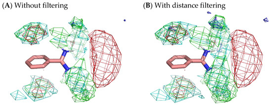
Figure 10.
Comparison of residue interaction profiles of benzamidine obtained from MSMD simulation with and without consideration of moving distance of probe molecules. (A) Without the selection of stable probe molecules (note that it is the same figure as Figure 4); (B) with the selection of stable probe molecules. Green, cyan, gray, blue, and red meshes indicate profiles of hydrophobic, hydrophilic, aromatic, basic, and acidic residues, respectively.
4.4. Substituent Evaluation with Residue Interaction Profiles
As mentioned in the Introduction, structural optimization that is strongly and specifically directed at a target protein is necessary in lead optimization. Residue interaction profiles can help the optimization step by suggesting whether a substituent is feasible for a protein binding pocket space. For instance, superimposing the interaction profile on a co-crystalized structure indicates how well the existing substituent matches the protein surface environment (Figure S2). Furthermore, residue interaction profiles of dozens of probes enable the establishment of a recommendation system by computational substitution of an initial compound and superimposition profiles of corresponding substituents or probes. Therefore, constructing residue interaction profiles of many probes with variation will enhance the impact in lead optimization processes.
5. Conclusions
In this article, we proposed inverse MSMD for analyzing a probe’s preference of interaction patterns. Unlike the analysis from known data, such as X-ray, Cryo-EM, and NMR structures, the method can process arbitrary probes, and the results are free from any chemical context of molecules. We assessed the method using benzamidine, catechol, and benzene, resulting in good agreement with the experimental structures. This method indicates where protein surfaces provide suitable binding sites for a probe and this, in turn, can be applied to lead optimization by suggesting substituents based on the vacant spaces of a binding pocket. More precisely, for a target protein surface where the next substituents on hit compounds are placed, the method provides information on which substituents are better in accordance with the residue interaction profiles of multiple probes or possible substituents. The next step in our method will involve proposing a quantitative metric of how well the residue environment and the residue interaction profile match. Furthermore, the construction of the residue interaction profile database is effective for the computational lead optimization process because the profiles can be applied to arbitrary proteins.
Supplementary Materials
The following supporting information can be downloaded at https://www.mdpi.com/article/10.3390/ijms23094749/s1.
Author Contributions
Conceptualization, K.Y., R.Y. and T.H.; methodology, K.Y., R.Y. and T.H.; software, K.Y.; formal analysis, K.Y., R.Y., G.K. and T.H.; writing—original draft preparation, K.Y. and R.Y.; writing—review and editing, K.Y., R.Y., G.K. and T.H.; supervision, T.H. All authors have read and agreed to the published version of the manuscript.
Funding
This research was partially funded by KAKENHI (20K19917, 22H03684) from the Japan Society for the Promotion of Science (JSPS); the Platform Project for Supporting Drug Discovery and Life Science Research (Basis for Supporting Innovative Drug Discovery and Life Science Research (BINDS)) (JP22ama121029) from the Japan Agency for Medical Research and Development (AMED); and the Program for Building Regional Innovation Ecosystems “Program to Industrialize an Innovative Middle Molecule Drug Discovery Flow through Fusion of Computational Drug Design and Chemical Synthesis Technology” from the Ministry of Education, Culture, Sports, Science and Technology (MEXT).
Data Availability Statement
The implementation and experimental data are open-sourced at https://github.com/keisuke-yanagisawa/exprorer_msmd (accessed on 22 April 2022) under the MIT license.
Acknowledgments
The authors thank Yutaka Akiyama at the Tokyo Institute of Technology for the constructive discussion and feedback. The computational experiments were performed using a TSUBAME3.0 supercomputer at the Tokyo Institute of Technology, for which we thank the institution.
Conflicts of Interest
The authors declare no conflict of interest.
References
- Berdigaliyev, N.; Aljofan, M. An overview of drug discovery and development. Future Sci. 2020, 12, 939–947. [Google Scholar] [CrossRef]
- Yoshino, R.; Yasuo, N.; Inaoka, D.K.; Hagiwara, Y.; Ohno, K.; Orita, M.; Inoue, M.; Shiba, T.; Harada, S.; Honma, T.; et al. Pharmacophore Modeling for Anti-Chagas Drug Design Using the Fragment Molecular Orbital Method. PLoS ONE 2015, 10, e0125829. [Google Scholar] [CrossRef]
- Yoshino, R.; Yasuo, N.; Hagiwara, Y.; Ishida, T.; Inaoka, D.K.; Amano, Y.; Tateishi, Y.; Ohno, K.; Namatame, I.; Niimi, T.; et al. In silico, in vitro, X-ray crystallography, and integrated strategies for discovering spermidine synthase inhibitors for Chagas disease. Sci. Rep. 2017, 7, 6666. [Google Scholar] [CrossRef] [Green Version]
- Chiba, S.; Ikeda, K.; Ishida, T.; Gromiha, M.M.; Taguchi, Y.-H.; Iwadate, M.; Umeyama, H.; Hsin, K.-Y.; Kitano, H.; Yamamoto, K.; et al. Identification of potential inhibitors based on compound proposal contest: Tyrosine-protein kinase Yes as a target. Sci. Rep. 2015, 5, 17209. [Google Scholar] [CrossRef] [PubMed] [Green Version]
- Chiba, S.; Ishida, T.; Ikeda, K.; Mochizuki, M.; Teramoto, R.; Taguchi, Y.-H.; Iwadate, M.; Umeyama, H.; Ramakrishnan, C.; Thangakani, A.M.; et al. An iterative compound screening contest method for identifying target protein inhibitors using the tyrosine-protein kinase Yes. Sci. Rep. 2017, 7, 12038. [Google Scholar] [CrossRef]
- Cavasotto, C.N.; Di Filippo, J.I. Artificial intelligence in the early stages of drug discovery. Arch. Biochem. Biophys. 2021, 698, 108730. [Google Scholar] [CrossRef] [PubMed]
- Liu, X.; IJzerman, A.P.; van Westen, G.J.P. Computational Approaches for De Novo Drug Design: Past, Present, and Future. In Methods in Molecular Biology; Cartwright, H., Ed.; Humana: New York, NY, USA, 2021; Volume 2190, pp. 139–165. [Google Scholar] [CrossRef]
- Lin, X.; Li, X.; Lin, X. A Review on Applications of Computational Methods in Drug Screening and Design. Molecules 2020, 25, 1375. [Google Scholar] [CrossRef] [PubMed] [Green Version]
- Kimber, T.B.; Chen, Y.; Volkamer, A. Deep Learning in Virtual Screening: Recent Applications and Developments. Int. J. Mol. Sci. 2021, 22, 4435. [Google Scholar] [CrossRef] [PubMed]
- Maia, E.H.B.; Assis, L.C.; Oliveira, T.A.; Silva, A.M.; Taranto, A.G. Structure-Based Virtual Screening: From Classical to Artificial Intelligence. Front. Chem. 2020, 8, 343. [Google Scholar] [CrossRef]
- Barelier, S.; Eidam, O.; Fish, I.; Hollander, J.; Figaroa, F.; Nachane, R.; Irwin, J.J.; Shoichet, B.K.; Siegal, G. Increasing Chemical Space Coverage by Combining Empirical and Computational Fragment Screens. ACS Chem. Biol. 2014, 9, 1528–1535. [Google Scholar] [CrossRef] [Green Version]
- Tidten-Luksch, N.; Grimaldi, R.; Torrie, L.S.; Frearson, J.A.; Hunter, W.N.; Brenk, R. IspE Inhibitors Identified by a Combination of In Silico and In Vitro High-Throughput Screening. PLoS ONE 2012, 7, e35792. [Google Scholar] [CrossRef] [Green Version]
- Chen, D.; Ranganathan, A.; IJzerman, A.P.; Siegal, G.; Carlsson, J. Complementarity between in Silico and Biophysical Screening Approaches in Fragment-Based Lead Discovery against the A2A Adenosine Receptor. J. Chem. Inf. Model. 2013, 53, 2701–2714. [Google Scholar] [CrossRef]
- Damm-Ganamet, K.L.; Bembenek, S.D.; Venable, J.W.; Castro, G.G.; Mangelschots, L.; Peeters, D.C.G.; Mcallister, H.M.; Edwards, J.P.; Disepio, D.; Mirzadegan, T. A Prospective Virtual Screening Study: Enriching Hit Rates and Designing Focus Libraries to Find Inhibitors of PI3Kδ and PI3Kγ. J. Med. Chem. 2016, 59, 4302–4313. [Google Scholar] [CrossRef] [PubMed]
- Fujitani, H.; Tanida, Y.; Matsuura, A. Massively parallel computation of absolute binding free energy with well-equilibrated states. Phys. Rev. E 2009, 79, 021914. [Google Scholar] [CrossRef] [PubMed]
- Abel, R.; Wang, L.; Harder, E.D.; Berne, B.J.; Friesner, F.A. Advancing Drug Discovery through Enhanced Free Energy Calculations. Acc. Chem. Res. 2017, 50, 1625–1632. [Google Scholar] [CrossRef]
- Kuhn, M.; Firth-Clark, S.; Tosco, P.; Mey, A.S.J.S.; Mackey, M.; Michel, J. Assessment of Binding Affinity via Alchemical Free-Energy Calculations. J. Chem. Inf. Model. 2020, 60, 3120–3130. [Google Scholar] [CrossRef]
- Ryde, U.; Söderhjelm, P. Ligand-Binding Affinity Estimates Supported by Quantum-Mechanical Methods. Chem. Rev. 2016, 116, 5520–5566. [Google Scholar] [CrossRef] [PubMed] [Green Version]
- Berman, H.; Henrick, K.; Nakamura, H.; Markley, J.L. The worldwide Protein Data Bank (wwPDB): Ensuring a single, uniform archive of PDB data. Nucleic Acids Res. 2007, 35, D301–D303. [Google Scholar] [CrossRef] [Green Version]
- Imai, Y.N.; Inoue, Y.; Yamamoto, Y. Propensities of Polar and Aromatic Amino Acids in Noncanonical Interactions: Nonbonded Contacts Analysis of Protein−Ligand Complexes in Crystal Structures. J. Med. Chem. 2007, 50, 1189–1196. [Google Scholar] [CrossRef]
- Wang, L.; Xie, Z.; Wipf, P.; Xie, X.-Q. Residue Preference Mapping of Ligand Fragments in the Protein Data Bank. J. Chem. Inf. Model. 2011, 51, 807–815. [Google Scholar] [CrossRef]
- Kasahara, K.; Shirota, M.; Kinoshita, K. Comprehensive Classification and Diversity Assessment of Atomic Contacts in Protein–Small Ligand Interactions. J. Chem. Inf. Model. 2013, 53, 241–248. [Google Scholar] [CrossRef]
- Zariquiey, F.S.; Souza, J.V.; Bronowska, A.K. Cosolvent Analysis Toolkit (CAT): A robust hotspot identification platform for cosolvent simulations of proteins to expand the druggable proteome. Sci. Rep. 2019, 9, 19118. [Google Scholar] [CrossRef] [Green Version]
- Ghanakota, P.; van Vlijmen, H.; Sherman, W.; Beuming, T. Large-Scale Validation of Mixed-Solvent Simulations to Assess Hotspots at Protein−Protein Interaction Interfaces. J. Chem. Inf. Model. 2018, 58, 784–793. [Google Scholar] [CrossRef]
- Schmidt, D.; Boehm, M.; McClendon, C.L.; Torella, R.; Gohlke, H. Cosolvent-Enhanced Sampling and Unbiased Identification of Cryptic Pockets Suitable for Structure-Based Drug Design. J. Chem. Theory Comput. 2019, 15, 3331–3343. [Google Scholar] [CrossRef]
- Kimura, S.R.; Hu, H.P.; Ruvinsky, A.M.; Sherman, W.; Favia, A.D. Deciphering Cryptic Binding Sites on Proteins by Mixed-Solvent Molecular Dynamics. J. Chem. Inf. Model. 2017, 57, 1388–1401. [Google Scholar] [CrossRef]
- Soga, S.; Shirai, H.; Kobori, M.; Hirayama, N. Identification of the Druggable Concavity in Homology Models Using the PLB Index. J. Chem. Inf. Model. 2007, 47, 2287–2292. [Google Scholar] [CrossRef] [PubMed]
- Jacobson, M.P.; Pincus, D.L.; Rapp, C.S.; Day, T.J.F.; Honig, B.; Shaw, D.E.; Friesner, R.A. A Hierarchical Approach to All-Atom Protein Loop Prediction. Proteins Struct. Funct. Genet. 2004, 55, 2287–2292. [Google Scholar] [CrossRef] [PubMed] [Green Version]
- Olsson, M.H.M.; Sondergaard, C.R.; Rostkowski, M.; Jensen, J.H. PROPKA3: Consistent treatment of internal and surface residues in empirical pKa predictions. J. Chem. Theory Comput. 2011, 7, 525–537. [Google Scholar] [CrossRef] [PubMed]
- Salomon-Ferrer, R.; Case, D.A.; Walker, R.C. An overview of the Amber biomolecular simulation package. Wiley Interdiscip. Rev. Comput. Mol. Sci. 2013, 3, 198–210. [Google Scholar] [CrossRef]
- Frisch, M.J.; Trucks, G.W.; Schlegel, H.B.; Scuseria, G.E.; Robb, M.A.; Cheeseman, J.R.; Scalmani, G.; Barone, V.; Petersson, G.A.; Nakatsuji, H.; et al. Gaussian 16; Revision B.01; Gaussian Inc.: Wallingford, CT, USA, 2016. [Google Scholar]
- Yanagisawa, K.; Moriwaki, Y.; Terada, T.; Shimizu, K. EXPRORER: Rational Cosolvent Set Construction Method for Cosolvent Molecular Dynamics Using Large-Scale Computation. J. Chem. Inf. Model. 2021, 61, 2744–2753. [Google Scholar] [CrossRef]
- Martínez, L.; Andrade, R.; Birgin, E.G.; Martínez, J.M. PACKMOL: A package for building initial configurations for molecular dynamics simulations. J. Comput. Chem. 2009, 30, 2157–2164. [Google Scholar] [CrossRef]
- Jorgensen, W.L.; Chandrasekhar, J.; Madura, J.D.; Impey, R.W.; Klein, M.L. Comparison of simple potential functions for simulating liquid water. J. Chem. Phys. 1983, 79, 926–935. [Google Scholar] [CrossRef]
- Hess, B. P-LINCS: A parallel linear constraint solver for molecular simulation. J. Chem. Theory Comput. 2008, 4, 116–122. [Google Scholar] [CrossRef] [PubMed]
- Bussi, G.; Donadio, D.; Parrinello, M. Canonical sampling through velocity rescaling. J. Chem. Phys. 2007, 126, 014101. [Google Scholar] [CrossRef] [Green Version]
- Bussi, G.; Parrinello, M. Stochastic thermostats: Comparison of local and global schemes. Comput. Phys. Commun. 2008, 179, 26–29. [Google Scholar] [CrossRef] [Green Version]
- Bussi, G.; Zykova-Timan, T.; Parrinello, M. Isothermal-isobaric molecular dynamics using stochastic velocity rescaling. J. Chem. Phys. 2009, 130, 074101. [Google Scholar] [CrossRef] [PubMed] [Green Version]
- Berendsen, H.J.C.; Postma, J.P.M.; Van Gunsteren, W.F.; Dinola, A.; Haak, J.R. Molecular dynamics with coupling to an external bath. J. Chem. Phys. 1984, 81, 3684–3690. [Google Scholar] [CrossRef] [Green Version]
- Abraham, M.J.; Murtola, T.; Schulz, R.; Páll, S.; Smith, J.C.; Hess, B.; Lindahl, E. Gromacs: High performance molecular simulations through multi-level parallelism from laptops to super-computers. SoftwareX 2015, 1–2, 19–25. [Google Scholar] [CrossRef] [Green Version]
- Shirts, M.R.; Klein, C.; Swails, J.M.; Yin, J.; Gilson, M.K.; Mobley, D.L.; Case, D.A.; Zhong, E.D. Lessons learned from comparing molecular dynamics engines on the SAMPL5 dataset. J. Comput. Aided Mol. Des. 2017, 31, 147–161. [Google Scholar] [CrossRef] [PubMed] [Green Version]
- Parrinello, M.; Rahman, A. Polymorphic transitions in single crystals: A new molecular dynamics method. J. Appl. Phys. 1981, 52, 7182–7190. [Google Scholar] [CrossRef]
- MacKerell, A.D., Jr.; Jo, S.; Lakkaraju, S.K.; Lind, C.; Yu, W. Identification and characterization of fragment binding sites for allosteric ligand design using the site identification by ligand competitive saturation hotspots approach (SILCS-Hotspots). Biochim. Biophys. Acta Gen. Subj. 2020, 1864, 129519. [Google Scholar] [CrossRef]
- Cock, P.J.A.; Antao, T.; Chang, J.T.; Chapman, B.A.; Cox, C.J.; Dalke, A.; Friedberg, I.; Hamelryck, T.; Kauff, F.; Wilczynski, B.; et al. Biopython: Freely available Python tools for computational molecular biology and bioinformatics. Bioinformatics 2009, 25, 1422–1423. [Google Scholar] [CrossRef] [PubMed]
- Richard, D.T.; Malcolm, M.C.; Alastair, D.G.L. Rings in drugs. J. Med. Chem. 2014, 57, 5845–5859. [Google Scholar] [CrossRef]
- Harder, M.; Kuhn, B.; Diederich, F. Efficient Stacking on Protein Amide Fragments. ChemMedChem 2013, 8, 397–404. [Google Scholar] [CrossRef] [PubMed]
- Ghanakota, P.; DasGupta, D.; Carlson, H.A. Free Energies and Entropies of Binding Sites Identified by MixMD Cosolvent Simulations. J. Chem. Inf. Model. 2019, 59, 2035–2045. [Google Scholar] [CrossRef] [PubMed]


Publisher’s Note: MDPI stays neutral with regard to jurisdictional claims in published maps and institutional affiliations. |
© 2022 by the authors. Licensee MDPI, Basel, Switzerland. This article is an open access article distributed under the terms and conditions of the Creative Commons Attribution (CC BY) license (https://creativecommons.org/licenses/by/4.0/).