Article

Monitoring and Evaluation of the Corrosion Behavior in Seawater of the Low-Alloy Steels BVDH36 and LRAH36

1
Competences Centre—Interfaces-Tribocorrosion-Electrochemical Systems (CC-ITES), “Dunărea de Jos” University of Galati, 47 Domneasca Street, RO-800008 Galati, Romania
2
Faculty of Medicine and Pharmacy, “Dunărea de Jos” University of Galați, 35 Al. I. Cuza Street, RO-800010 Galati, Romania
*
Author to whom correspondence should be addressed.
Int. J. Mol. Sci. 2024, 25(12), 6405; https://doi.org/10.3390/ijms25126405
Submission received: 7 April 2024 / Revised: 18 May 2024 / Accepted: 5 June 2024 / Published: 10 June 2024
(This article belongs to the Section Physical Chemistry and Chemical Physics)

Abstract

:
The purpose of this study is to evaluate the corrosion resistance in natural seawater (Năvodari area) of two types of low-alloy carbon steels BVDH36 and LRAH36 by electrochemical methods. The electrochemical methods used were the evolution of the free potential (OCP), electrochemical impedance spectroscopy (EIS), polarization resistance (Rp) and corrosion rate (Vcorr), potentiodynamic polarization (PD), and cyclic voltammetry (CV). The studies were completed by ex situ characterization analyzes of the studied surfaces before and after corrosion such as: optical microscopy, scanning electron microscopy and X-ray diffraction analysis. The results of the study show us that the polarization resistance of the low-alloy carbon steel BVDH36 is higher compared to the polarization resistance of the low-alloy carbon steel LRAH36. It is also observed that with the increase in the immersion time of the samples in natural seawater, the polarization resistance of the BVDH36 alloy increases over time and finally decreases, and for the carbon steel LRAH36 the polarization resistance increases.

1. Introduction

In a world where metals and metal alloys are indispensable, corrosion appears as one of the most serious problems of modern society and the resulting losses every year are of the order of trillions of dollars [1]. Regarding the corrosion losses, approximately 90% are related to ferrous materials, used in the construction of road bridges, reinforcements, rolling stock and agricultural equipment, maritime ships, and port facilities [2]. In second and third place in the hierarchy of practical use are aluminum and copper alloys, which are also subject to corrosion [2]. Marine corrosion is a permanent problem, not only for moving or stationary ships, but also for all port installations, desalination installations, and objects that come into prolonged contact with water and the marine atmosphere [3,4,5,6,7,8,9,10]. The corrosivity of seawater depends on many factors such as salinity, dissolved oxygen, temperature, biological factors, and the material subject to corrosion, etc. [8]. Depending on the metallic material subjected to the action of seawater, all these factors can also determine the type of corrosion that can occur [8]. Corrosion in the marine environment can manifest in various forms and takes place through electron transfer reactions [8]. That is why predicting the lifetime of a material used in a certain application is particularly important to avoid accidental and catastrophic failures [3,4,5,6,7,8,9,10]. The deep sea is the direction of oceanic exploration due to the wealth of oil, gas, and minerals. In the last decade, a new challenge is focused on the study of the reliability of deep engineering equipment [11,12,13,14]. There has been interest in using low-alloy steels for deep-sea applications due to their excellent mechanical properties, general corrosion resistance, biocompatibility, and weldability in the marine environment [15,16]. Low-alloy steel usually protects other metallic materials by corroding as a sacrificial anode due to the negative self-corrosion potential [17,18,19]. Wei et al. [20] highlighted the fact that low-alloy steels with a carbon content of less than 0.2% by weight, to which Cu, Cr, Ni, P, Si, and Mn are mainly added as alloying elements up to a total of at most 5% by weight, are inexpensive and widely used in marine engineering such as ship plates, sea crossing bridges, and submarine pipelines [20]. However, the marine environment is the most corrosive natural environment, and the service performance of low-alloy steels in marine environments can be difficult to guarantee [20]. Therefore, there is a need to improve the corrosion resistance of low-alloy steels for marine engineering. According to the literature data, it is known that the corrosion resistance of low-alloy steel is closely related to the alloying elements, but the research conclusions are mainly qualitative, such as the following: the corrosion resistance of low-alloy steel will improve with the increase in the content of Cr [20]. Thus, authors such as Jia et al. [21] provided more information on the mechanical properties of low-alloy steel subjected to uniform and pitting corrosion. This study was conducted because in recent times more and more emphasis has been placed on the use of high-strength low-alloy steel [21,22] in the development of long-lasting tall structures or in other special structures, since they contribute to the reduction in element sizes, especially the thickness of the plates. However, if these low-alloy steel structures were to serve in a harsh environment such as a high humidity and salinity atmosphere, they would be exposed to a severe threat of degradation as a result of the corrosion process. In the case of atmospheric corrosion of structures, pitting corrosion and uniform corrosion are very common. However, pitting corrosion is more harmful because it has random characteristics and the maximum stress always occurs at the location of the maximum corrosion depth [23]. Pitting corrosion would induce the degradation of tensile strength [24,25,26,27,28], compressive strength [25,26,27,29,30], flexural strength [24,26,31,32,33], and shear strength [34] of low-alloy steel plate [35]. Also, the reduction in strength is also mainly related to the corrosion process with an effect on the damage of the minimum cross-section. Thus, pitting corrosion leads to a rough surface and contributes to a severe stress concentration [23,36,37], causing a reduction in deformability. The authors [21] highlighted that the prediction relationship of surface roughness and deformability reduction could be described by a parabolic law [24,27]. The location and dimensions of the pitting affect the tensile characteristic and failure mode of the steel plate under load [29]. In this context, Jia et al. [21] performed several copper acetate accelerated spray corrosion tests for high-strength low-alloy steel plate samples. The authors performed the tensile tests in order to investigate the mechanical properties of the low-alloy steel plate before and after corrosion, aiming at the main parameters of corrosion time and tensile prestressing. The study was carried out to establish the relationship between the degradation effects of the low-alloy steel structures due to the two types of corrosion and the analyzed mechanical properties. The experimental results showed that as the corrosion time increased, the total corrosion loss of the unprestressed samples continued to increase with a gradually decreasing corrosion rate. In addition, during corrosion, the roughness experienced an upward trend, and the lower surface was rougher than the upper surface. Separating the corrosion components, the total corrosion loss was dominated by pitting corrosion, although the proportion of uniform corrosion increased more and more. Regarding long-term corrosion, the authors [21] showed that elastic tensile prestressing can lead to some inhibition of pitting corrosion while contributing to the easy development of uniform corrosion. The results of this study [21] showed that compared to the unprestressed specimens, the tensile mechanical and deformation characteristics of the tensile elastically prestressed specimens were both slightly improved. Considering the effects of the two types of corrosion on the mechanical properties, Jia et al. showed that uniform corrosion mainly affected tensile mechanical characteristics, while pitting corrosion is predominantly attributed to deformation performance degradation [21]. Zhang et al. pointed out that the poor corrosion resistance of steel can affect the stability and safety of the material. Therefore, it is extremely important to explore the corrosion behavior of low-alloy steel for practical applications [38]. According to the literature data, it is known that many factors affect the corrosion resistance of low-alloy steels, such as: alloy content [39,40], Cl concentration [41,42], O2 content [43,44], corrosion environment [45,46], heat treatment [47,48], and grain size [49,50]. Zhang et al. [38] investigated the effect of tempering temperature on the corrosion of low-alloy steel. Low-alloy steel is mainly supplied in an annealed condition. Although tempering is an effective method of improving the mechanical properties of steel, its influence on corrosion behavior has been controversial. Therefore, Zhang et al. [38] studied the effects of different tempering temperatures on the corrosion resistance of low-alloy steel in humid atmosphere using an immersion test, a salt spray test, electrochemical measurements, morphological characterization, and phase analysis. The results showed that the defects and highly reactive nature of the high angle grain boundaries of “bare” steels are preferentially corroded. In the initial stage of corrosion, the annealing temperature affects the distribution of small-angle grain boundaries. The annealed specimens corroded slightly due to the low interface energy. In the later stage of corrosion, Zhang et al. [38] observed that the corrosion resistance of the analyzed samples still depends on the matrix due to the limited protection of the rust layer. Thus, the load transfer resistance improves and the corrosion resistance becomes better as the annealing temperature decreases. Chen et al. [51] studied literature data on the corrosion mechanism of low-alloy steel in a tropical coastal atmosphere. The authors highlighted in their study that the atmospheric corrosion process is an electrochemical process that occurs when a thin layer of electrolyte forms on the metal surface [52]. The liquid layer with airborne salt species (e.g., chlorides and carbonates) dissolving in coastal atmospheres can greatly increase the corrosion rate of low-alloy steel, especially in tropical regions characterized by a high temperature and relative humidity [53,54,55]. The role of chlorides in the coastal atmospheric corrosion process is extremely complicated and there are several possible mechanisms of acceleration: (a) hygroscopic chlorides would absorb moisture from the atmosphere and thus favor the formation of electrolytes, lowering the relative humidity threshold for corrosion in the atmosphere [56,57]; (b) some chloride rust phases are soluble and therefore the electrolyte conductivity would have increased considerably, which in turn accelerates the atmospheric corrosion process [51]; (c) Cl (chloride ions) would favor phase transformations in the deposited corrosion products (rust) and therefore could modify the protective functions [58,59]. Based on the information presented above, the authors [51] pointed out that chlorides influence not only the corrosion rate, but also the constituents of the corrosion products. In general, the main corrosion products of low-alloy steel are lepidocrocite (γ-FeOOH) and goethite (α-FeOOH) under low or no Cl exposure [60,61]. Akaganeite (β-FeOOH) and maghemite (γ-Fe2O3)/magnetite (Fe3O4) could be produced by the hydrolysis of ferrous chloride (FeCl2) and oxidation of the low-alloy steel substrate relative to a large amount of chloride deposition [62,63]. Among the aforementioned rust phases, the compact and denser α-FeOOH is of critical importance in reducing atmospheric corrosion [59]. Compared to other corrosion products, β-FeOOH is electrochemically active and tends to form thick layers in corrosion products favoring the formation of cracks in these corrosion products as well as localized attack on the surface of low-alloy steel [64,65,66,67,68]. Based on the results of the study [51], it was indicated that a high rate of chloride deposition would reduce the protective capacity of the rust layer due to an increase in the content of harmful akaganeite (β-FeOOH) and maghemite (γ-Fe2O3) in the corrosion products. Also, the existence of the corrosion products β-FeOOH and γ-Fe2O3 induced the appearance of pits due to severe pitting corrosion on the surface of low-alloy steel. Quantitatively, strong positive correlations were obtained between the chloride deposition rate, the corrosion rate, and the protective ability index of the rust layer by means of the Pearson correlation coefficient. Thus, the rate of chloride deposition could be directly related to the protection of the rust layer as well as the corrosion severity of low-alloy steel in the tropical coastal atmosphere [51]. The objective of this work is to study the corrosion behavior in natural seawater (Black Sea) of two types of steel (BVDH36 and LRAH36) used in the Galati and Constanţa shipyards for the construction of different parts of maritime ships. In recent years, studies have been reported in the specialized literature that deal more with the influence of technological and mechanical parameters on the corrosion resistance of different types of steel immersed in solutions simulating the marine environment [69,70,71,72,73,74,75,76,77,78,79,80]. But it can be seen that there is a lack of studies regarding the comparison between two types of materials immersed in natural seawater that are focused on obtaining a clearer vision of the corrosion resistance of these types of materials. The paper presents the study of the corrosion behavior of the two steels by electrochemical methods such as the free potential, electrochemical impedance spectroscopy, potentiodynamic polarization, and cyclic voltammetry.

2. Results and Discussion

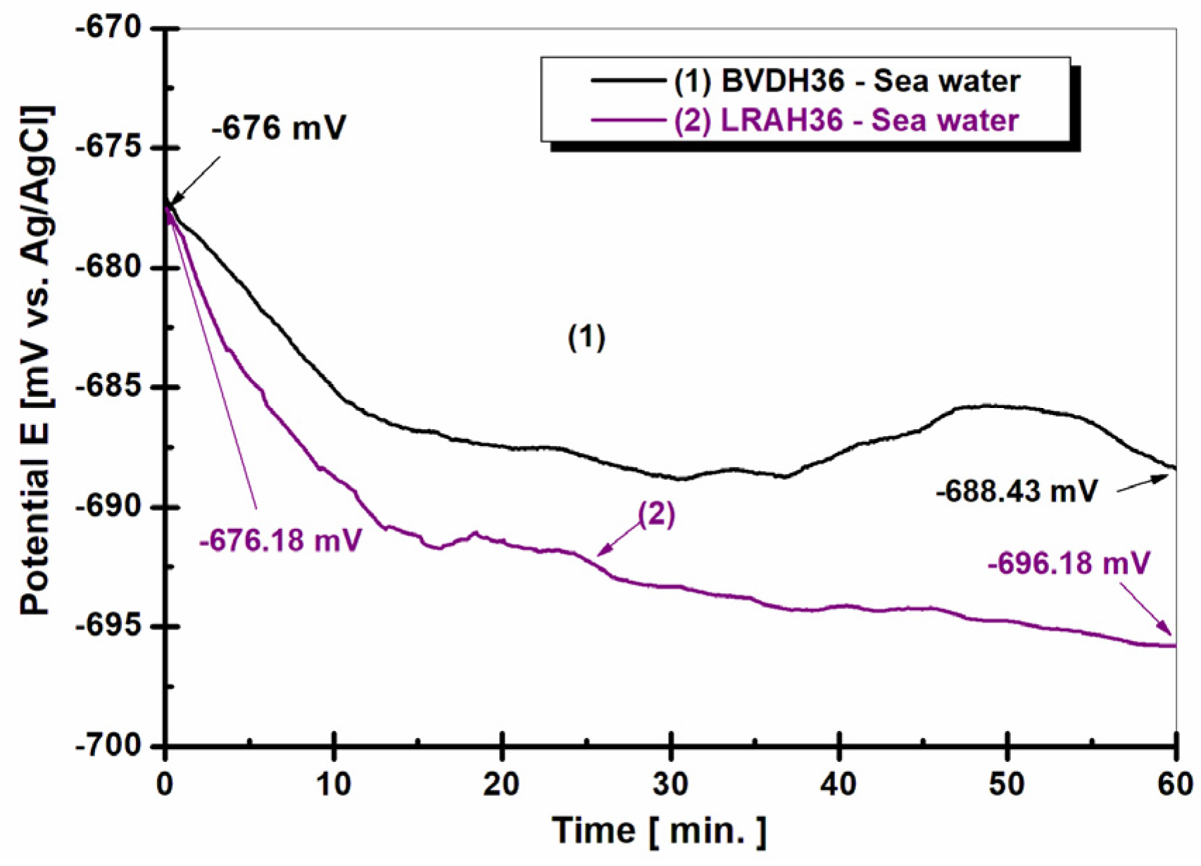
2.1. The Evolution of the Free Potential

Figure 1 shows the evolution of the free potential for the two types of studied materials immersed in natural seawater for 60 min.
From Figure 1, it can be seen that both low-alloy steels tend to move the free potential towards negative values; thus, for BVDH36 steel, the value of the initial potential is E = −676 ± 12 mV vs. Ag/AgCl, after one hour reaching the value E = −688.43 ± 21 mV vs. Ag/AgCl. For LRAH36 steel, at immersion it has the value of E = −676.18 ± 35 mV vs. Ag/AgCl, and after one hour of immersion in seawater the value of the free potential is E = −696.18 ± 31 mV vs. Ag/AgCl, at 20 mV vs. Ag/AgCl more negative than the immersion value.
The tendency of the potential to move towards more negative values indicates that there is a dissolution of the oxide layer formed on the surface of the studied materials [3,4,5,6,7,8,9,10], with this behavior leading to a decrease in the corrosion resistance of the materials.
Comparing the seawater immersion behavior of the two steels, it is observed that LRAH36 steel immersed in seawater has a tendency to move towards more negative values, more pronounced compared to BVDH36 steel immersed in seawater. Upon immersion, the value of the free potential for LRAH36 steel immersed in seawater is ∆E = 0.18 mV more negative than the free potential value obtained for BVDH36 steel immersed in seawater. At the end of the 60 min, the difference between the two steels should be a little higher than the value from the immersion. The potential difference between the two steels at the end of the free potential evolution measurement is only 7.75 mV.

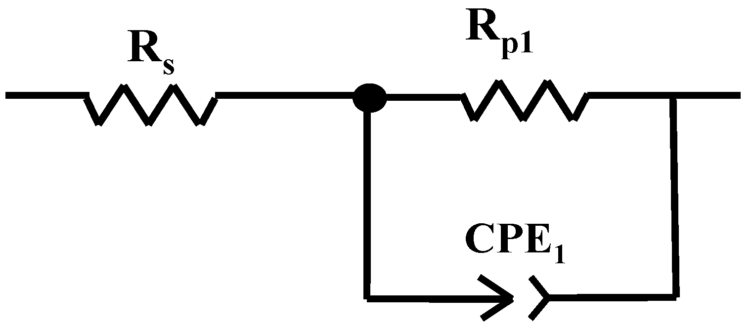
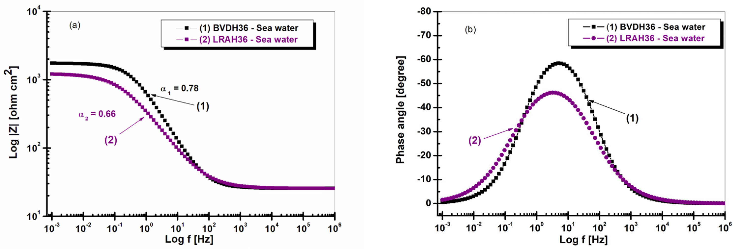
2.2. Electrochemical Impedance Spectroscopy (EIS) after 1 h of Immersion

The electrochemical impedance spectroscopy (EIS) method is a modern method of studying the processes that take place in an electrochemical cell [9,10]. From an electrical point of view, any cell behaves as an ohmic resistor in a direct current and as an impedance in an alternating current [9,10]. This method consists of disturbing the system with an alternating signal superimposed on the direct current that normally supplies the cell and measuring the response. Thus, the cell can be connected in an alternating current bridge that allows the impedance to be determined [9,10].
Figure 2 shows the Nyquist diagram for the two types of studied steel immersed in natural seawater after one hour’s of immersion.
From Figure 2, it can be seen that BVDH36 steel has a little better polarization resistance, Rp = 1733.77 ohm cm2, which means a higher corrosion resistance compared to LRAH36, which has a weaker polarization resistance of Rp = 1208.63 ohm cm2. To obtain the values of the polarization resistance, the experimental data were fitted with the Zview software version 3.4 using a Randles circuit. The equivalent circuit used to fit the experimental data is shown in Figure 3.
The Randles circuit is a simple circuit that is composed of a bias resistor (Rp), being connected in parallel with the constant phase element (CPE), which replaces the capacity of the ideal capacitor created due to the formation of the electric double layer, in parallel. The circuit is connected in series with the solution resistance (Rs) representing the resistance of the electrolyte and the resistance of the electrical conductors but also other external resistances of the cell connected in series [9,10].
In the case of the BVDH36 equivalent circuit, the solution resistance is Rs = 25.52 ohm. This circuit has a constant phase element, the electrochemical potential capacity, CPE1 = 0.00031058 F/cm2, and the angle α1 = 0.78 (can be seen in Figure 4a).
For the LRAH36 equivalent circuit, the solution resistance is Rs = 25.48 ohm. The circuit has a constant phase element, namely the electrochemical potential, CPE1 = 0.00076669 F/cm2 and the angle α2 = 0.66 (can be seen in Figure 4a).
Figure 4a,b show the Bode diagrams of the two low-alloy steels, BVDH36 and LRAH36, immersed in seawater.
Figure 4a has a high impedance value obtained at low frequency, and medium frequency reveals a low reactivity or good corrosion resistance for BVDH36 steel. Figure 4b shows the phase angle as a function of frequency. It can be observed that the maximum value of the phase angle of −63 degrees, which is obtained in the case of BVDH36 steel, compared to LRAH36 steel which has a phase angle of −46 degrees. Figure 4 further demonstrates that the corrosion resistance of the BVDH36 steel sample is better as compared to the LRAH36 steel sample.

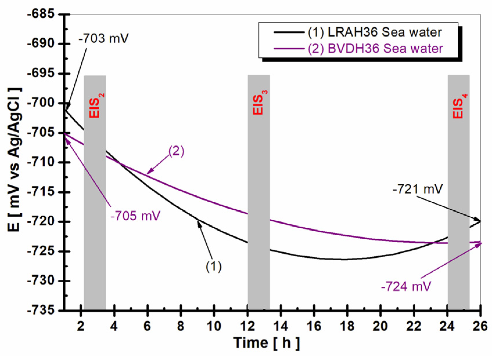
2.3. Evolution of Open Circuit Potential in Seawater for 26 h of LRAH36 Steel and BVDH36 Steel

Figure 5 shows the evolution of the free potential of BVDH36 and LRAH36 steels immersed in natural seawater for a period of 26 h.
Analyzing the data in Figure 5, it can be seen that the open circuit potential trend during the 26 h of immersion the BVDH36 steel has a less negative trend than LRAH36. As seen at the beginning of the corrosion test, the initial dip value is E = −705 ± 12 mV vs. Ag/AgCl, reaching the value E = −724 ± 15 mV vs. Ag/AgCl.
In the case of LRAH36 steel, the open circuit potential during the 26 h moves towards more negative values, starting from the initial potential E = −703 ± 33 mV vs. Ag/AgCl and reaching after 26 h the value E = −721 ± 28 mV vs. Ag/AgCl.
The continuous negative trend of the open circuit potential during the 26 h of immersion for both low-alloy steels BVDH36 and LRAH36 is attributed to the inability of the steels to retain corrosion products on their surface, which could function as protective layers of oxides.

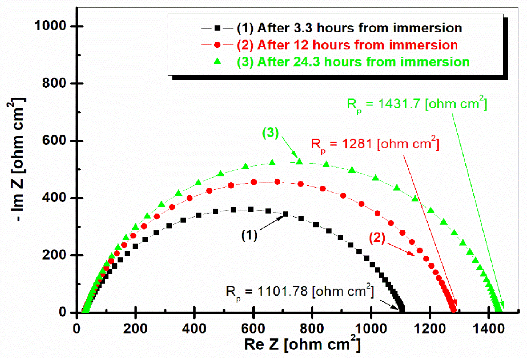
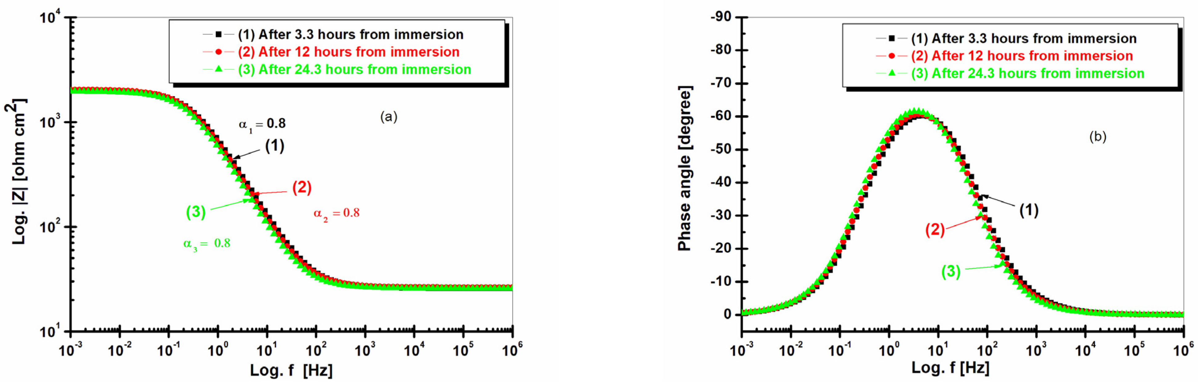
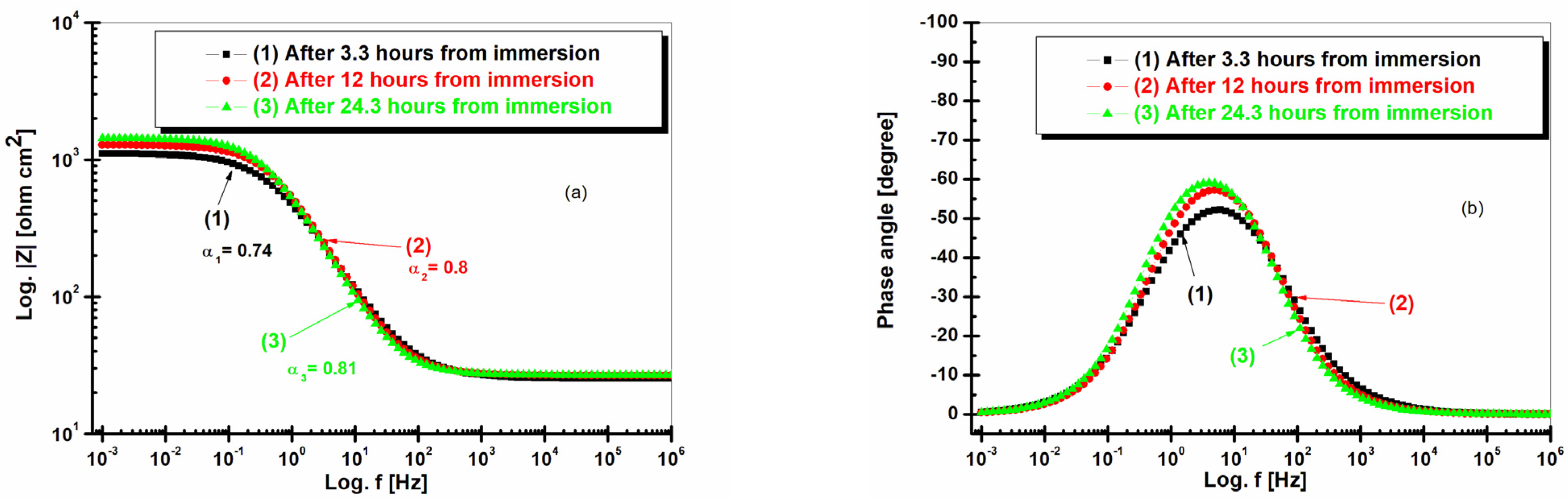
2.4. Electrochemical Impedance Spectroscopy (EIS) after 3.3 h, 12 h, and 24.3 h of Immersion in Seawater of LRAH36 and BVDH36 Steel Samples

Figure 6 shows electrochemical impedance spectroscopy in the form of a Nyquist representation for BVDH36 steel immersed in natural seawater at different time intervals.
From Figure 6, it can be seen that in the superimposed Nyquist impedances from BVDH36 steel the polarization resistance increases and finally decreases. So that after 3.3 h of immersion it has a polarization resistance of 2003.62 ohm cm2. After 12 h of immersion the polarization resistance value is a little higher being 2031.56 ohm cm2. The value decreases after 24.3 h of immersion in seawater, having the polarization resistance of 1943.5 ohm cm2.
Figure 7 shows the electrochemical impedance spectroscopy in the form of a Nyquist representation for LRAH36 steel immersed in natural seawater at different time intervals.
From Figure 7, it can be seen that the polarization resistance increases over time, along with the number of impedances; thus, after 3.3 h of immersion it has the lowest polarization resistance of 1101.78 ohm cm2, reaching after 24.3 h of immersion in seawater the highest polarization resistance at 1431.7 ohm cm2.
Comparing Figure 6 and Figure 7, it can be seen that BVDH36 steel has a higher polarization resistance, compared to LRAH36 steel, which has a lower polarization resistance, that is, a weaker corrosion resistance.
Figure 8 shows the electrochemical impedance spectroscopy as a Bode representation for BVDH36 steel immersed in natural seawater at different time intervals.
From Figure 8a, it can be seen that BVDH36 steel with Bode diagrams after 3.3 h of immersion, after 12 h of immersion and after 24.3 h of immersion in seawater, respectively, has an impedance well above 103 ohm cm2 between the frequencies 103 and 101.2 Hz, and the impedance decreases after 3.3 h of immersion, after 12 h of immersion, and after 24.3 h of immersion, being 10 ohm cm2 between the frequencies of 102 and 106 Hz. The angles for Bode diagrams after 3.3 h, 12 h, and 24.3 h of immersion are the same with α1 = α2 = α3 = 0.8. From Figure 8b of BVDH36 steel, it can be seen that in the Bode diagrams after 3.3 h of immersion, after 12 h of immersion, and after 24.3 h of immersion, respectively, the phase angle attains the value of −67 degrees.
Figure 9 shows the electrochemical impedance spectroscopy in the form of a Bode representation for LRAH36 steel immersed in natural seawater at different time intervals.
In Figure 9a, LRAH36 steel in Bode diagrams after 3.3 h of immersion, after 12 h of immersion, and after 24.3 h of immersion in seawater has maximum impedances slightly above 103 ohm cm2 between the frequencies of 103 and 101.3 Hz, and the impedance drops to 10 ohm cm2 between the frequencies of 102 and 106 Hz. From Figure 9a, LRAH36 steel has maximum impedances slightly above 103 ohm cm2, after 3.3 h of immersion, after 12 h of immersion, and after 24.3 h of immersion, respectively, which leads to the conclusion that BVDH36 steel is a little more resistant to corrosion than LRAH36 steel, where BVDH36 steel, from Figure 8a of the Bode diagrams after 3.3 h of immersion, after 12 h of immersion, and after 24.3 h of immersion, respectively, can be seen to have a maximum impedance well above 103 ohm cm2. The depressed angles are observed in Figure 9a, with α1 = 0.74 after 3.3 h of immersion, α2 = 0.8 after 12 h of immersion, and α3 = 0.81 after 24.3 h of immersion.
From Figure 9b, it can be seen that LRAH36 steel after 3.3 h of immersion has a maximum phase angle of −53 degrees, after 12 h of immersion has a phase angle of approximately −59 degrees, and after 24.3 h of immersion has a phase angle of −63 degrees.

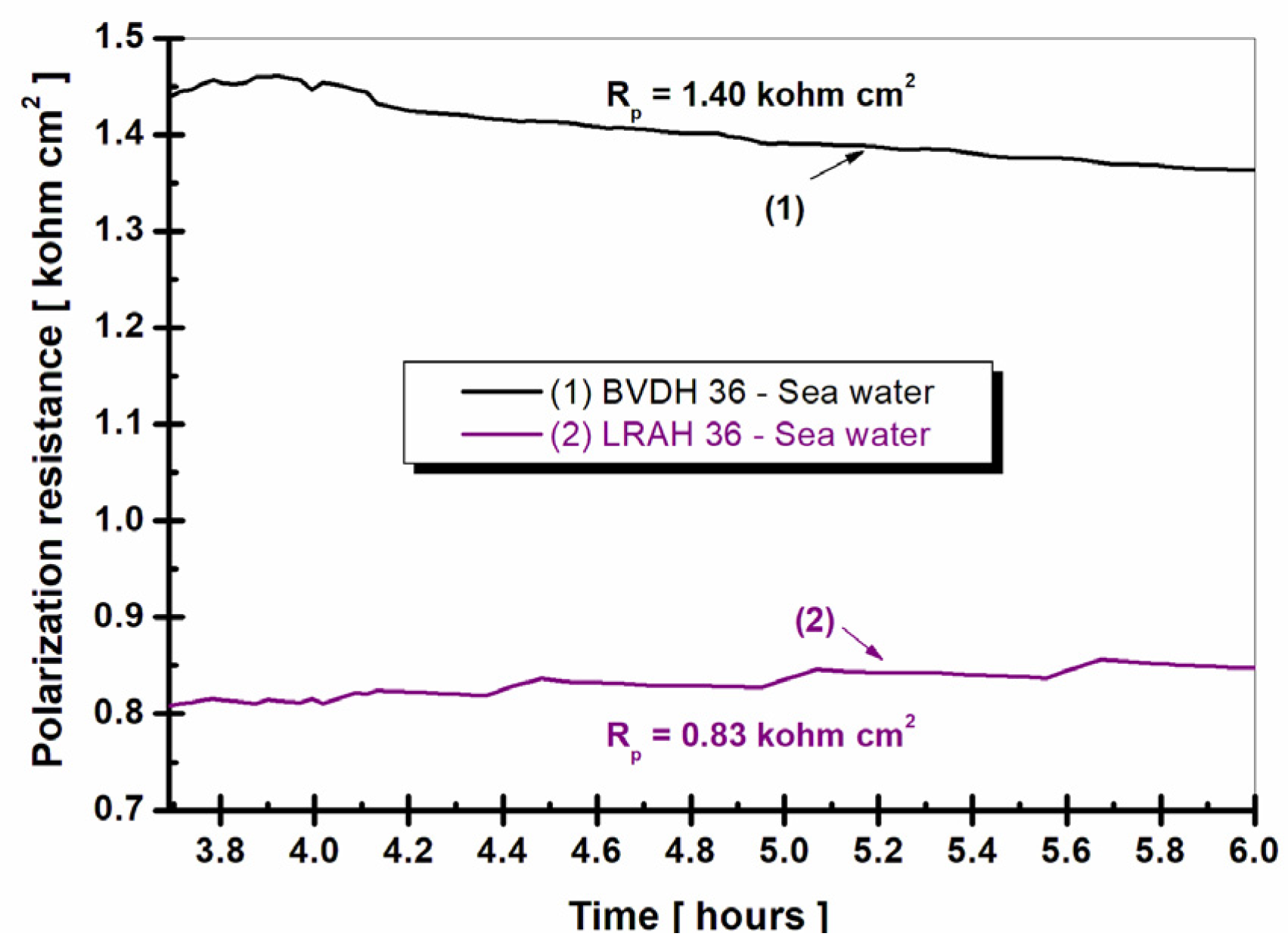
2.5. Polarization Resistance and Corrosion Rate

Figure 10 shows the evolution over time of the polarization resistance in natural seawater of BVDH36 and LRAH36 steels.
Polarization resistance and corrosion rate are evaluated by the linear polarization method by plotting 100 linear polarization curves.
Using the 100 polarization curves by plotting the Tafel slopes with Stern Geary equation [3], as the Equations (1) and (2), 100 values of polarization resistances and 100 values of corrosion rate were calculated for each alloy on each measurement step.
R p = B i c o r r = ( Δ E ) ( Δ i ) Δ E 0
B = b a b c 2.3 ( b a + b c )
where
Rp is the polarization resistance;
icorr the corrosion current density;
The proportionality constant, B, for a particular system can be determined as shown by Stern and Geary, calculated from ba and bc, the slopes of the anodic and cathodic Tafel, Equation (2).
From the analysis of Figure 10, it can be seen that the average value of the polarization resistance in the case of BVDH36 steel is approximately two times higher than the value obtained by LRAH36 steel. At the same time, it is well known in the specialized literature that the polarization resistance is inversely proportional to the corrosion rate; in other words, the higher the polarization resistance for a studied material, the lower the corrosion rate.
Figure 11 shows the evolution over time of the corrosion rate as the penetration rate into natural seawater of BVDH36 and LRAH36 steel.
From the analysis of Figure 11, it can be seen that the average value of the corrosion rate in the case of BVDH36 steel is approximately two times lower than the value obtained by LRAH36 steel. If for BVDH36 steel we have a value of Vcorr = 87 µm/year, for LRAH36 steel we have a value of Vcorr = 146.64 µm/year, thus indicating that BVDH36 steel has a higher corrosion resistance compared to LRAH36 steel immersed in natural seawater.

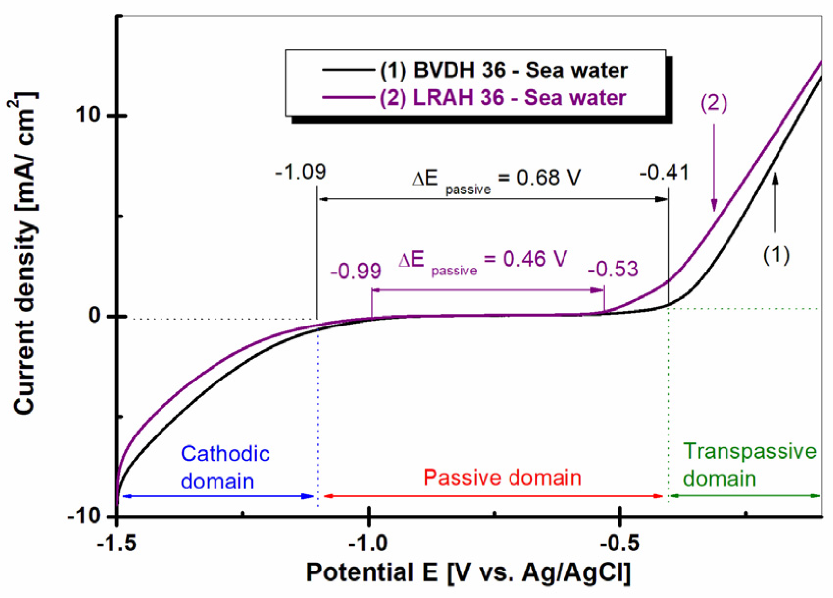
2.6. Potentiodynamic Polarization Plots, Logarithmically Scaled for Current Density, Obtained in Seawater for Steels BVDH36 and LRAH36 (Tafel Representation)

Figure 12 shows the Tafel curves for BVDH36 and LRAH36 steels immersed in natural seawater.
As can be seen from the polarization diagrams shown in Figure 13, the corrosion potentials show a shift towards negative values for both low-alloy steels. The lowest value of the Ecorr corrosion potential was recorded in the case of BVDH36 steel (−904.2 mV (vs. Ag/AgCl)), which indicates that BVDH36 steel is slightly more resistant in seawater compared to LRAH36 steel (−925.6 mV (vs. Ag/AgCl)). The systematic evolution is in the following order: Ecorr: BVDH36 < LRAH36; and for icorr: BVDH36 (21.69 µA/cm2) < LRAH36 (14.41 µA/cm2). In general, the more positive the Ecorr value is, the more susceptible the material is to corrosion processes.
In order to investigate the effect of seawater on the passive range of BVDH36 and LRAH36 steel immersed in natural seawater, the potentiodynamic polarization curves were drawn, the results of which are presented in Figure 13.
As shown in Figure 13, curve (1), BVDH36 steel immersed in natural seawater shows a wide range of passivation between E1 = −1.09 V vs. Ag/AgCl and E2 = −0.41 V vs. Ag/AgCl, having a passivation range of ΔEpassiv = 0.68 V. The LRAH36 steel curve (2) immersed in natural seawater has a smaller passivation range compared to BVDH36 steel immersed in seawater which is between E3 = −0.99 V vs. Ag/AgCl and E4 = −0.53 V vs. Ag/AgCl, having a passivation range of ΔEpassiv = 0.46 V. The wider the passivation range of a material, the better the corrosion behavior.

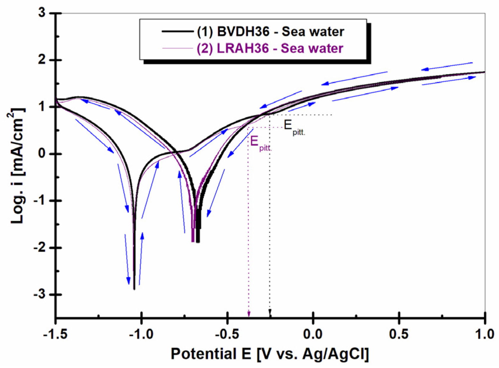
2.7. Cyclic Voltammetry

Figure 14 shows the cyclic voltammetry for BVDH36 and LRAH36 steels immersed in natural seawater.
From Figure 14, at the intersection of the inflection point, where the current density suddenly increases and changes its slope, the pitting corrosion potential of BVDH36 steel is Epit = −0.25 V and LRAH36 steel has the pitting corrosion potential Epit = −0.37 V. The more positive the pitting corrosion potential is, the more resistant it is to corrosion.

2.8. Optical Microscopy of BVDH36 and LRAH36 Steels before and after Corrosion

Figure 15 shows the optical microscopy for BVDH36 steel before and after the corrosion process.
Figure 16 shows the optical microscopy for LRAH36 steel before and after corrosion.
The optical microscopy images, presented in Figure 15b and Figure 16b, after corrosion highlight the occurrence of pitting corrosion being much more pronounced in the case of LRAH36 steel compared to BVDH36 steel.

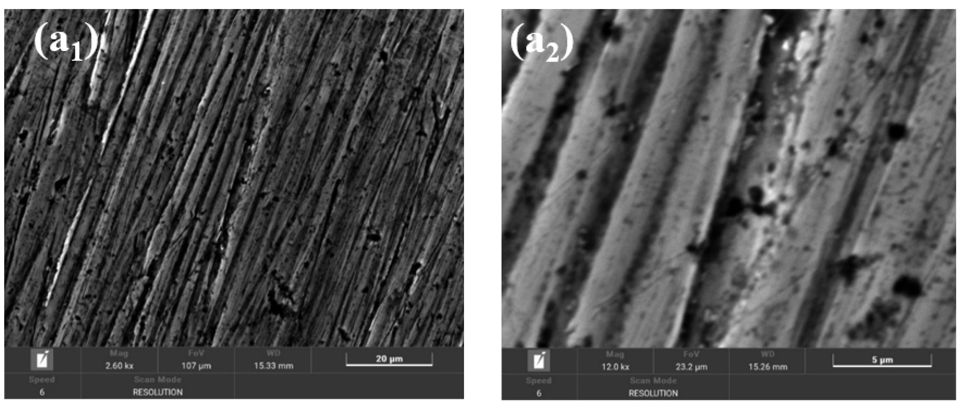
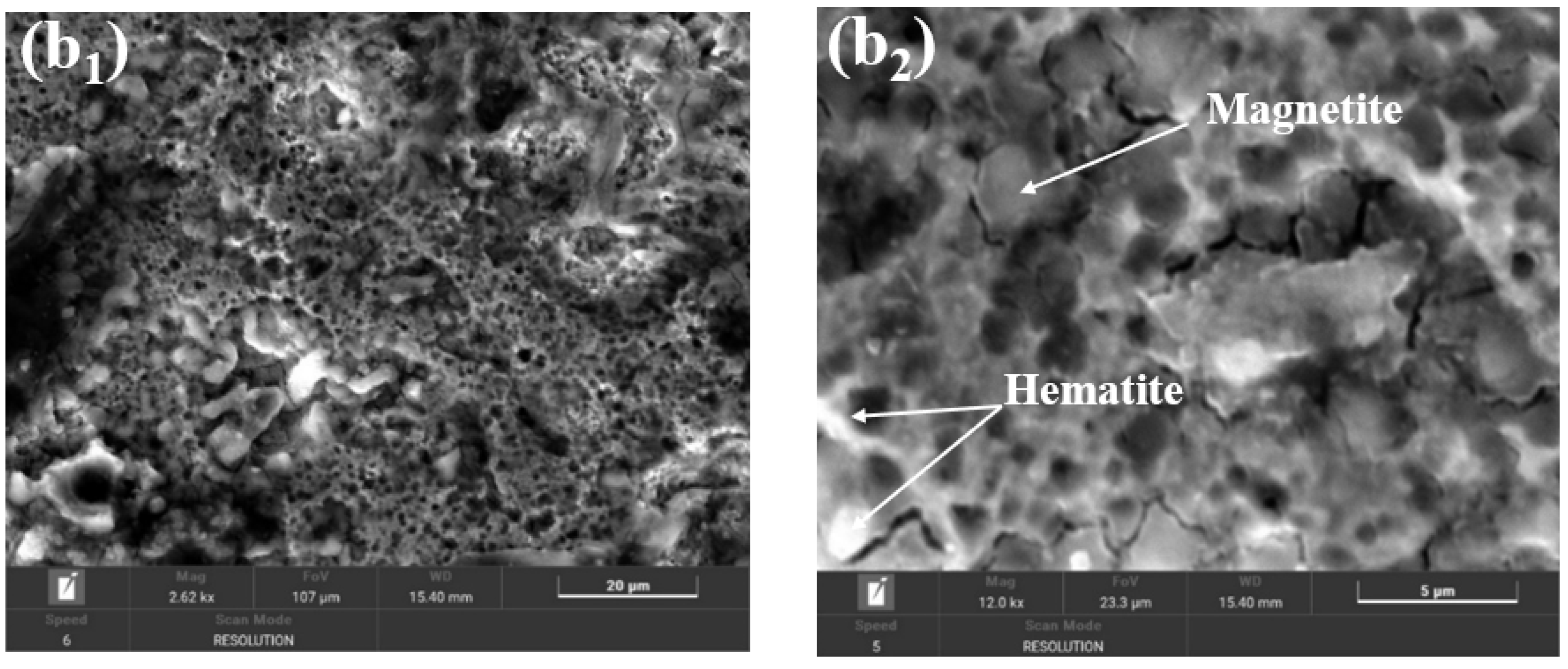
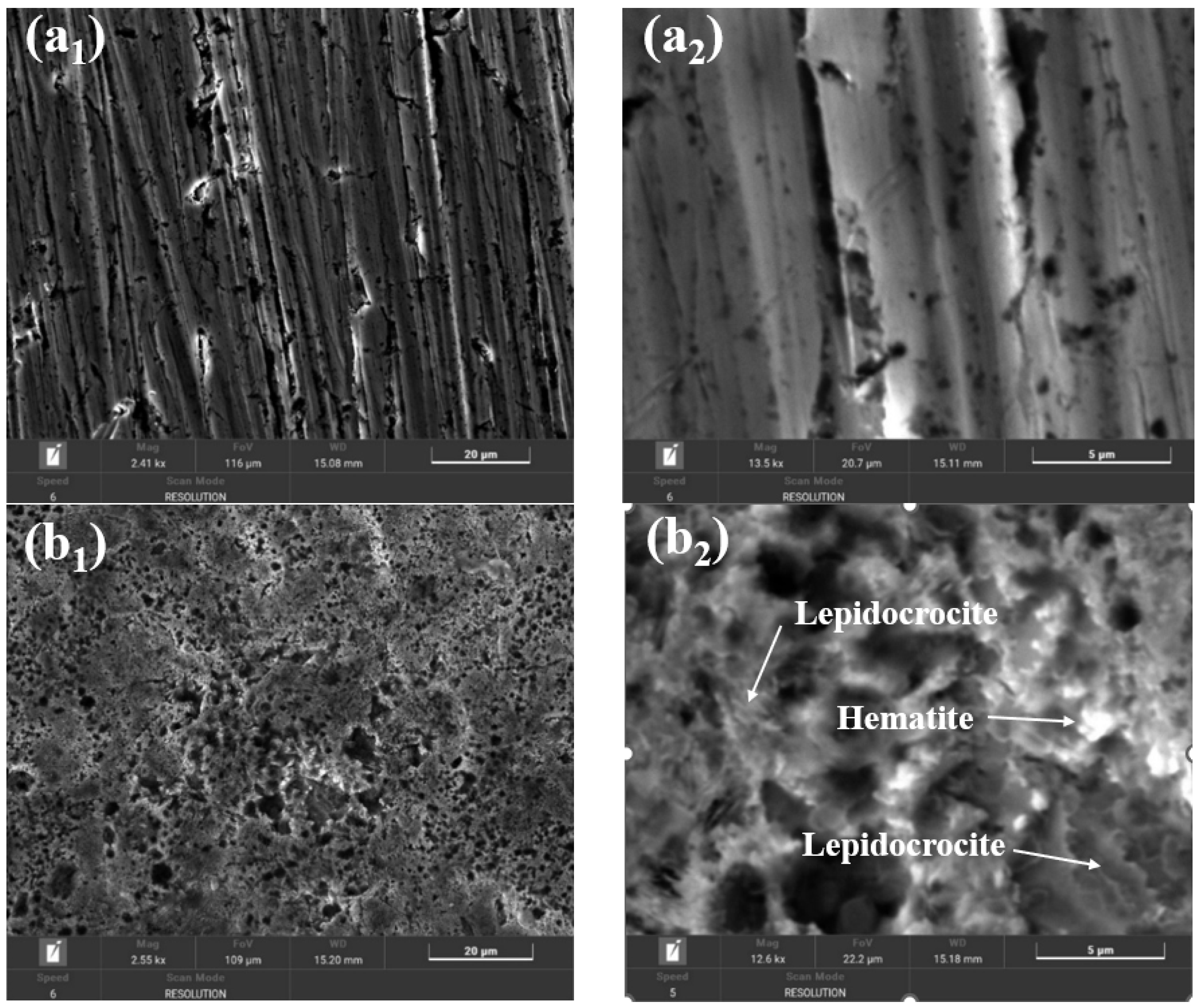
2.9. Morphological and Compositional Characterization of the Surfaces of BVDH36 and LRAH36 Steels before and after Corrosion by Scanning Electron Microscopy (SEM-EDX)

Figure 17 shows the SEM images of BVDH36 steel before (Figure 17a1,a2) and after the corrosion process (Figure 17b1,b2).
From Figure 17a2 it can be seen that BVDH36 steel before corrosion has a clean surface, without corrosion products, but with slight surface defects due to mechanical processing of surfaces. After the corrosion, the appearance of raised agglomerated formations associated with the corrosion products formed on the surface of BVDH36 steel immersed in natural seawater (Năvodari area) can be observed. Using the data from the specialized literature, from Figure 17b2 it is possible to identify hematite (Fe2O3) in the form of small spherical crystalline globules [19] and the appearance of dark flat surfaces of magnetite (Fe3O4) [20]. The formation of corrosion products is also confirmed by the data obtained from energy-dispersive X-ray spectroscopy (EDX) by the appearance of the element oxygen (Table 1).
From Table 1, of the EDX spectrum, for the BVDH36 sample, before corrosion we have the following mass fractions % by weight (Wt %): 90.2% Fe; 6.6% C; 1.7% Mn; 1.2% Si; 0.1% Ni; 0.1% P; and 0.1% Al, and atomic fractions (σ %): 1.3% Fe; 1.3% C; 0.1% Mn; 0.1% Si; 0.1% Ni; 0.1% P; and 0.1% Al.
From Table 2, of the EDX spectrum, for the BVDH36 sample, after corrosion we have the following mass fractions % by weight (Wt %): 68.5% Fe; 15.6% C; 14.8% O; 0.9% Mn; 0.1% Ni; and 0.1% Cu, and the corresponding atomic fractions (σ %): 0.6% Fe; 0.6% C; 0.3% O; 0.1% Mn; 0.1% Ni; and 01% Cu.
Comparing the data obtained from the two EDX spectra of the BVDH36 sample before corrosion (Table 1) and after corrosion (Table 2), it can be seen that after corrosion, the percentage of oxygen increases to the value of 14.3 Wt%, while the percentage of iron decreases from 90.2 Wt% before corrosion to 68.5 Wt% after corrosion, which confirms the appearance of some oxides on the surface of the sample.
The SEM morphology of the surface of the LRAH36 steel samples before and after corrosion is shown in Figure 18. As with the BVDH36 sample (Figure 17a1,a2), in Figure 18a1,a2 it can be seen that the surface of the LRAH36 steel before corrosion is clean, without corrosion products, but with slight surface defects due to mechanical processing activities. Comparing the morphologies of the two low-alloy steels after corrosion (Figure 17b1,b2) with Figure 18b1,b2, it is observed that the surface of the LRAH36 steel is covered by an almost uniform layer of corrosion products, a layer which covers the entire surface of the steel. The formation of corrosion products is also confirmed by the data obtained from the EDX spectrum, by the appearance of the oxygen element (Table 3).
Based on the data from the specialty literature regarding the analysis of the surface morphology of the corrosion products [19,20], the following corrosion products were identified: hematite in the form of small spherical crystalline globules and lepidocrocite with a laminar “bird’s nest” appearance and lepidocrocite in the form of flower petals.
The results obtained by the energy-dispersive X-ray spectroscopy (EDX) technique are shown in Table 3 and Table 4.
From Table 3, of the EDX spectrum, for sample LRAH36, before corrosion, we have the following mass fractions % by weight (Wt %): 91.5 Fe; 6% C; 1.6% Mn; 0.5% Si; 0.2% Mo; 0.1% Ni; and 0.1% Al, and atomic fractions (σ %): 1.3% Fe; 1.2% C; 0.1% Mn; 0.1% Si; 0.3% Mo; 0.1% Ni; and 0.1% Al.
From Table 4, of the EDX spectrum, for sample LRAH36, after corrosion we have the following mass fractions % by weight (Wt %): 80.7% Fe; 10.8% C; 6.4% O; 1.2% Mn; 0.3% Cu; 0.3% Si; 0.1% Ni; 0.1% Al; and 0.1% P, and corresponding atomic fractions (σ %): 0.7% Fe; 0.8% C; 0.3% O; 0.1 Mn; 0.1% Cu; 0.1% Si; 0.1% Ni; 0.1% Al; and 0.1% P. From the comparative analysis of the two EDX spectra (Table 3 and Table 4) corresponding to the LRAH36 low-alloy steel samples, it was found that in the case of the LRAH36 sample after corrosion, the percentage of oxygen increases to a value of 6.4 Wt%, while the percentage of iron decreases from a value of 91.5 Wt% before corrosion (Table 3) to a value of 80.7 Wt% after corrosion (Table 4).

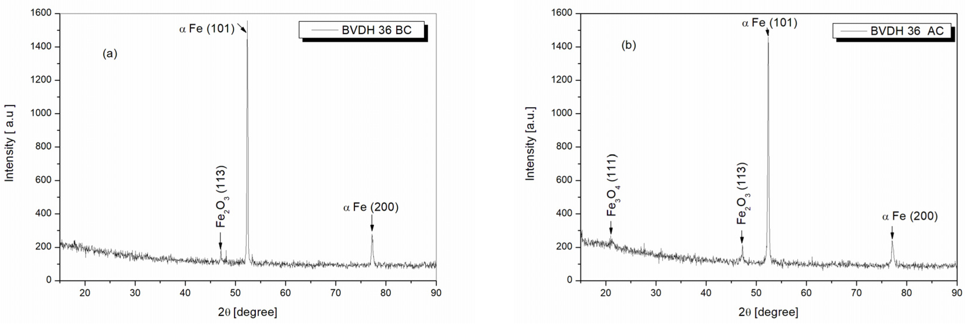
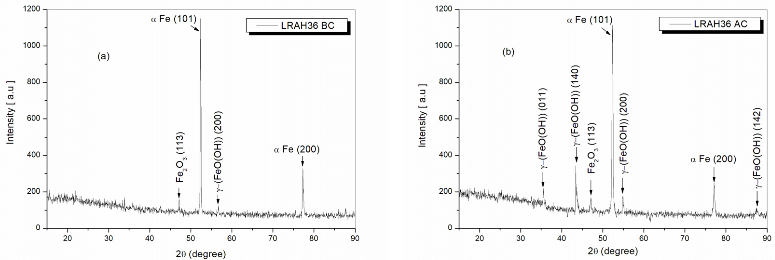
2.10. Structural Analysis of BVDH36 and LRAH36 Steels before and after Corrosion Using the XRD Technique

Figure 19a,b show the X-ray diffractograms of BVDH36 steel samples before corrosion and after corrosion. Analyzing the ray diffractogram in Figure 19a, it was observed that for BVDH36 steel before corrosion, the dominant diffraction peak corresponds to the (101) plane identified at the 2θ angle of 52.35°. This diffraction peak belongs to the element α-Fe. Also, α-Fe was identified at the angle 2θ of 77.20°, but with the intensity of the diffraction peak corresponding to the lower (200) plane. The element α-Fe with the crystallographic planes (101 and 200) was identified using the card COD 96-110-0109. Next to the element α-Fe, identified using the card COD 96-210-8029, the compound Fe2O3 was observed at the angle 2θ of 47.20° with the crystallographic plane (113), but with the intensity of the diffraction peak being much lower than the intensities of the diffraction peaks belonging to the element α-Fe.
From the analysis of the X-ray diffractogram of BVDH36 steel after corrosion shown in Figure 19b, it is observed that the diffraction peaks identified before corrosion are preserved, respectively, for the element α-Fe and compound Fe2O3 (hematite) at the same 2θ diffraction angles with the same crystallographic planes. However, compared with the BVDH36 steel sample before corrosion, in the case of BVDH36 steel after corrosion, it can be seen that the intensities of the two diffraction peaks corresponding to the element α-Fe are lower, while the intensity of the hematite diffraction peak Fe2O3 increases 1.6 times, and in addition the compound Fe3O4 (magnetite) appears at the 2θ angle of 21.44° related to the crystallographic plane (111) identified with the card COD 96-900-2321. The results obtained from the XRD data (Figure 19) are in good agreement with those obtained from SEM-EDX images.
Table 5 shows the centralized data obtained by the X-ray diffraction technique of the two low-alloy steels BVDH36 and LRAH36, before corrosion and after corrosion in natural seawater.
Figure 20 shows the X-ray diffractograms of the LRAH36 steel samples before corrosion (Figure 20a) and after corrosion (Figure 20b).
From Figure 20a, in the case of LRAH36 steel before corrosion, the following crystalline phases were identified: the compound Fe2O3 at the angle of 47.20° with the crystallization plane (113) using the card COD 96-210-8029; the element α-Fe with planes (101) and (200) using COD 96-110-0109. Also, with the help of the card COD 96-901-5157, the compound γ-FeO(OH) (lepidocrocite) was also identified at the 2θ angle of 54.97°, having the crystallographic plane (200).
From the analysis of the X-ray diffraction spectrum in Figure 20b, it is observed that in the case of the LRAH36 sample after corrosion, the diffraction peaks identified before corrosion on the same type of sample studied show, respectively, the elements α-Fe and hematite Fe2O3 at the same 2θ diffraction angles and with the same crystallographic planes.
Also, as in the case of BVDH36 steel after corrosion, it can be seen that the intensities of the two diffraction peaks corresponding to the element α-Fe are lower, while the intensity of the diffraction peak of hematite increased 1.8 times. It should be noted that in addition to the sample studied before corrosion (Figure 20a), in the case of this sample (Figure 20b), the corrosion product, lepidocrocite, appears as γ-(FeO(OH)) at the following diffraction angles 2θ: 35.53°, 43.70°, 54.97°, and 87.58°, with the crystallographic planes (011, 140, 200, 142) identified with the card COD 96-901-5157.
The results obtained from the XRD investigation (Figure 20) are in good agreement with those obtained from the SEM-EDX images, confirming that the rust layer in the case of LRAH36 steel consists of the lepidocrocite compound γ-FeO(OH) and hematite Fe2O3, with the observation that the corrosion product lepidocrocite is in a greater proportion than hematite.

3. Materials and Methods

3.1. Materials

For this study, two types of low-alloy steels in the naval field (BVDH36 and LRAH36) purchased from the Galati (Liberty, Galati, Romania) steel plant were used. The composition of the two steels is shown in Table 6 and Table 7.
To carry out the electrochemical tests, the steel samples were cut to the size of 2.5 cm × 2.5 cm × 3 mm, glued with a copper wire to have electrical contact, and embedded in epoxy resin to be able to have a well-defined active surface: the steel BVDH36 had an area of 2.52 cm2 and the steel LRAH36 had an area of 2.55 cm2. Before each experiment, the samples were sanded with SiC 1200# abrasive paper to remove the oxide layer formed on their surface, then cleaned and rinsed with distilled water.

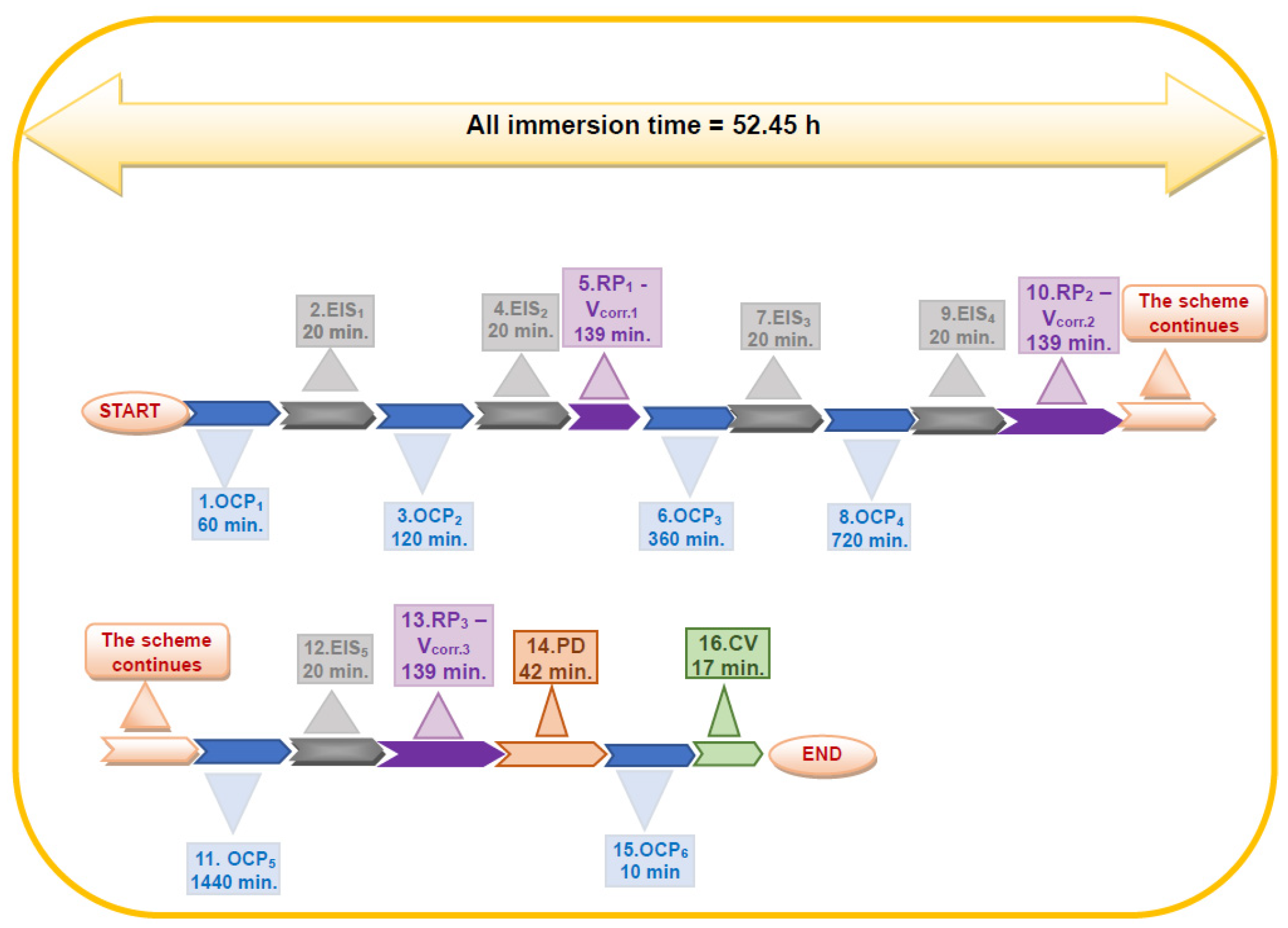
3.2. Electrochemical Test

The PGZ 100 electrochemical equipment was used, on which the VoltaMaster 4 software version 5.1 was running. The electrochemical tests were performed at room temperature, 25 ± 1 °C, in an electrochemical cell composed of three electrodes. The working electrode (WE) is the tested steel sample of BVDH36 and LRAH36. The counter electrode (CE) is formed by a Pt-Rh grid, and the reference electrode (RE) is Ag/AgCl with saturated KCl solution that has a potential of +199 mV vs. NHE. The volume of electrolyte used for each experiment was 150 mL (natural seawater from the Black Sea, Năvodari, România). The physicochemical characteristics of natural seawater measured before the electrochemical tests using a multiparameter Consort C533 are presented in Table 8.
To determine the corrosion resistance of low-alloy steels immersed in natural seawater, the following experimental protocol is applied (Figure 21).
1. OCP1—Open circuit potential 1, 4 s measurement period, 1 h duration.
2. EIS1—Electrochemical Impedance Spectroscopy 1—Frequency from 100 kHz to 100 mHz, AC = 10 mV, Freq./decade 20, duration 20 min.
3. OCP2—Open circuit potential 2, 4 s measurement period, 2 h duration.
4. EIS2—Electrochemical Impedance Spectroscopy 2—Frequency from 100 kHz to 100 mHz, AC = 10 mV, Freq./decade 20, duration 20 min.
5. Rp1—Vcor1–Bias resistance 1—Corrosion rate 1: ±40 mV, 100 points, 5 mV/s, duration 139 min.
6. OCP3—Open circuit potential 3, 4 s measurement period, 6 h duration.
7. EIS3– Electrochemical Impedance Spectroscopy 3—Frequency from 100 kHz to 100 mHz, AC = 10 mV, Freq./decade 20, duration 20 min.
8. OCP4—Open circuit potential 4, 4 s measurement period, 12 h duration.
9. EIS4—Electrochemical Impedance Spectroscopy 4—Frequency from 100 kHz to 100 mHz, AC = 10 mV, Freq./decade 20, duration 20 min.
10. Rp2—Vcor2–Polarization resistance 2—Corrosion rate 2: ±40 mV, 100 points, 5 mV/s, duration 139 min.
11. OCP5—Open circuit potential 5, 4 s measurement period, 24 h duration.
12. EIS5—Electrochemical Impedance Spectroscopy 5—Frequency from 100 kHz to 100 mHz, AC = 10 mV, Freq./decade 20, duration 20 min.
13. Rp3—Vcor3–Polarization resistance 3—Corrosion rate 3: ±40 mV, 100 points, 5 mV/s, duration 139 min.
14. PD—Potentiodynamic bias 1—from −1.5 V to 1.0 V; scan rate: 1 mV/s, sampling 1:4, duration 42 min.
15. OCP6—Open circuit potential 6, measurement period 4 s, duration 10 min.
16. CV—Cyclic voltammetry—from −1.5 V to 1.0 V to −1.5 V, scan speed: 5 mV/s, 1 cycle, duration 17 min.
The experimental results are presented using the Origin 2022 software version 9.9. Each experiment was repeated three times in order to check the reproducibility of the experimental results.

3.3. Characterization of Low-Alloy Steels before and after Electrochemical Tests

An OPTIKA XDS 3MET metallurgical optical microscope was used to highlight the surface morphology of the studied steels.
In order to obtain high-resolution detailed images of BVDH36 and LRAH36 steel samples before and after corrosion, the TESCAN scanning electron microscope was used. This scanning electron microscope is equipped with an EDX detector. Energy-dispersive X-ray spectroscopy (EDX) was used in this study to determine the elemental chemical composition. EDX data were processed using Bruker Esprit software v2.2, which enables easy EDX elemental chemical composition analysis and sample mapping.
In order to identify the crystalline phases of the studied steels, the X-ray diffraction technique was applied. Based on X-ray diffraction analysis recorded with Drone Test Equipment 3 using a Cobalt anode ( ), on the field between 15 and 90°, diffraction spectra were obtained, which were later matched using the standardized data of Match!3 software version 4.0 for phase identification (http://www.crystalimpact.com/match accessed on 6 March 2024), and the results were matched to the crystallographic database (Crystallography Open Database, COD), identifiable with a 9-digit code.

4. Conclusions

In this work, the corrosion behavior in Black Sea water of two low-alloy steels, BVDH36 and LRAH36, was studied for 52.45 h by electrochemical methods.
Comparing the seawater immersion behavior of the two steels, it is observed that LRAH36 steel immersed in seawater tends to move towards more negative, more pronounced values than BVDH36 steel immersed in seawater. During immersion, the free potential value for LRAH36 steel immersed in seawater is 0.18 mV vs. Ag/AgCl more negative than the free potential value obtained for BVDH36 steel immersed in seawater. After 60 min, the difference between the two steels is slightly greater than the value at immersion. Basically, the potential difference between the two steels at the end of the free potential evolution measurement is 7.75 mV compared to Ag/AgCl. The tendency of the potential to move towards more negative values indicates that there is a dissolution of the oxide layer formed on the surface of the studied materials, this behavior leading to a decrease in the corrosion resistance of the materials.
The continued trend towards negative values of the open circuit potential over 26 h of the low-alloy steels BVDH36 and LRAH36 is attributed to the inability of the steels to retain corrosion products on their surface, which could act as protective oxide layers.
From the plots in the Nyquist plot, it can be seen that LRAH36 steel is slightly weaker in corrosion due to its lower polarization resistance (EIS after 1 h of immersion has a polarization resistance of 1208.63 ohm cm2, with EIS after 24.3 h of immersion reaching a polarization resistance of 1431.7 ohm cm2), compared to BVDH36 steel, which has a higher corrosion resistance due to the higher value of polarization resistance (EIS after 1 h of immersion: polarization resistance of 1733.77 ohm cm2, with EIS after 12 h of immersion reaching the highest polarization resistance at 2031.56 ohm cm2).
From the Bode plots, it was observed that BVDH36 steel is slightly more resistant to corrosion as it has a maximum impedance of well above 103 ohm cm2 between the frequencies of 10−3 and 10−1.2 Hz and has a phase angle of about −67 degrees, compared with LRAH36 steel, which has a maximum impedance of just over 103 ohm cm2 and a phase angle of −63 degrees.
In potentiodynamic polarization diagrams, PD, BVDH36 steel has a higher passivation range than LRAH36 steel, which indicates that BVDH36 steel is more corrosion-resistant than LRAH36.
Corrosion in pitting is very dangerous because the pittings have small diameters, being hardly visible, but they are deep and can affect the structure of the steel. Based on the results obtained from the cyclic voltammetry, the more pronounced sensitivity of LRAH36 steel to pitting corrosion in seawater was highlighted compared to BVDH36 steel.
The results obtained from the SEM-EDX investigations are in good agreement with those obtained from the XRD data. Thus, for both samples of low-alloy steels before corrosion, BVDH36 and LRAH36, their surface is clean, without corrosion products, but with slight surface defects due to mechanical processing activities. In the case of BVDH36 steel after corrosion, the formed corrosion products are hematite Fe2O3 and magnetite Fe3O4. In the case of LRAH36 steel after corrosion, the entire surface of the steel is covered by an almost uniform layer of corrosion products, which consists of the compound lepidocrocite γ-FeO(OH) and hematite Fe2O3, with the observation that the corrosion product lepidocrocite is in a greater proportion than hematite.

Author Contributions

Conceptualization, L.B. and A.M.; methodology, L.B.; software, E.R.A.; validation, L.B.; formal analysis, L.B.; investigation, A.M.; resources, L.B. and E.R.A.; data curation, L.B.; writing—original draft preparation, A.M.; writing—review and editing, L.B. and E.R.A.; visualization, A.M.; supervision, L.B.; project administration, L.B.; funding acquisition, L.B.; XRD data analysis. All authors have read and agreed to the published version of the manuscript.

Funding

This work was supported by the UEFISCDI, Project ID—PN-III-P4-PCE-2021-0702, project number PCE 102/2022-2024.

Institutional Review Board Statement

Not applicable.

Informed Consent Statement

Not applicable.

Data Availability Statement

Data are contained within the article.

Acknowledgments

All the experimental work was performed at the Competences Center Interfaces—Tribocorrosion and Electrochemical Systems (CC-ITES)—and at the laboratories for Applied Electrochemistry for Materials and Environmental Science and Engineering (LEASIMM) and Electrochemistry and Corrosion (EC) at Dunarea de Jos University of Galati. The authors would like to express their appreciation to UEFISCDI—PN-III-P4-PCE-2021-0702 for the funding support.

Conflicts of Interest

The authors declare no conflicts of interest.

References

  1. Al-Moubaraki, A.H.; Obot, I.B. Corrosion challenges in petroleum refinery operations: Sources, mechanisms, mitigation, and future outlook. J. Saudi Chem. Soc. 2021, 25, 101370–101397. [Google Scholar] [CrossRef]
  2. Yan, L.; Deng, W.; Wang, N.; Xue, X.; Hua, J.; Chen, Z. Anti corrosion reinforcements using coating technologies—A Review. Polymers 2022, 14, 4782. [Google Scholar] [CrossRef] [PubMed]
  3. Benea, L.; Mardare, L.; Simionescu, N. Anticorrosion performances of modified polymeric coatings on E32 naval steel in sea water. Prog. Org. Coat. 2018, 123, 120–127. [Google Scholar] [CrossRef]
  4. Benea, L.; Simionescu, N.; Mardare, L. The effect of polymeric protective layers and the immersion time on the corrosion behavior of naval steel in natural seawater. J. Mater. Res. Technol. 2020, 9, 13174–13184. [Google Scholar] [CrossRef]
  5. Xu, Y.; Huang, Y.; Cai, F.; Lu, D.; Wang, X. Study on corrosion behavior and mechanism of AISI 4135 steel in marine environments based on field exposure experiment. Sci. Total Environ. 2022, 830, 154864. [Google Scholar] [CrossRef] [PubMed]
  6. Motlatle, A.M.; Ray, S.S.; Ojijo, V.; Scriba, M.R. Polyester-based coatings for corrosion protection. Polymers 2022, 14, 3413. [Google Scholar] [CrossRef] [PubMed]
  7. Gudić, S.; Vrsalović, L.; Matošin, A.; Krolo, J.; Oguzie, E.E.; Nagod, A. Corrosion behavior of stainless steel in seawater in the presence of sulfide. Appl. Sci. 2023, 13, 4366. [Google Scholar] [CrossRef]
  8. Melchers, R.E. Modelling long term corrosion of steel infrastructure in natural marine environments. In Understanding Biocorrosion Fundamentals and Applications, 1st ed.; Liengen, T., Féron, D., Basséguy, R., Beech, I.B., Eds.; Woodhead Publishing: Sawston, UK, 2014; pp. 213–241. [Google Scholar] [CrossRef]
  9. Plieth, W. Corrosion and Corrosion Protection. In Electrochemistry for Materials Science, 1st ed.; Plieth, W., Ed.; Elsevier: Amsterdam, The Netherlands, 2008; pp. 291–321. [Google Scholar] [CrossRef]
  10. Magar, H.S.; Hassan, R.Y.A.; Mulchandani, A. Electrochemical impedance spectroscopy (EIS): Principles, construction, and biosensing applications. Sensors 2021, 21, 6578. [Google Scholar] [CrossRef]
  11. Humooudi, A.; Hamoudi, M.R.; Ali, B.M. Corrosion mitigation in crude oil process by implementation of desalting unit in erbil refinery. ASRJETS 2017, 36, 224–241. [Google Scholar]
  12. Fan, W.; Zhang, Y.; Tian, H.; Wang, W.; Li, W. Corrosion behavior of two low alloy steel in simulative deep-sea environment coupling to titanium alloy. Colloids Interface Sci. Commun. 2019, 29, 40–46. [Google Scholar] [CrossRef]
  13. Brown, A.; Wright, R.; Mevenkamp, L.; Hauton, C. A comparative experimental approach to ecotoxicology in shallow-water and deep-sea holothurians suggests similar behavioural responses. Aquat. Toxicol. 2017, 191, 10–16. [Google Scholar] [CrossRef] [PubMed]
  14. Kark, S.; Brokovich, E.; Mazor, T.; Levin, N. Emerging conservation challenges and prospects in an era of offshore hydrocarbon exploration and exploitation. Conserv. Biol. J. Soc. Conserv. Biol. 2015, 29, 1573–1585. [Google Scholar] [CrossRef] [PubMed]
  15. Lubinevsky, H.; Hyams-Kaphzan, O.; Almogi-Labin, A.; Silverman, J.; Harlavan, Y.; Crouvi, O.; Herut, B.; Kanari, M.; Tom, M. Deep-sea soft bottom infaunal communities of the Levantine Basin (SE Mediterranean) and their shaping factors. Mar. Biol. 2017, 164, 36. [Google Scholar] [CrossRef]
  16. Azumi, K.; Yamamoto, G.; Seo, M. Pursuit of electronic property change of the passive film on titanium. Zairyo-To-Kankyo 2009, 46, 176–179. [Google Scholar] [CrossRef]
  17. Finšgar, M.; Jackson, J. Application of corrosion inhibitors for steels in acidic media for the oil and gas industry: A review. Corros. Sci. 2014, 86, 17–41. [Google Scholar] [CrossRef]
  18. Chen, Y.Y.; Tzeng, H.J.; Wei, L.I.; Wang, L.H.; Oung, J.C.; Shih, H.C. Corrosion resistance and mechanical properties of low-alloy steels under atmospheric conditions. Corros. Sci. 2005, 47, 1001–1021. [Google Scholar] [CrossRef]
  19. Xing, S.H.; Li, Y.; Wharton, J.A.; Fan, W.J.; Liu, G.Y.; Zhang, F.; Zhao, X.D. Effect of dissolved oxygen and coupled resistance on the galvanic corrosion of Cr-Ni lowalloy steel/90-10 cupronickel under simulated deep sea condition. Mater. Corros. 2017, 68, 1123–1128. [Google Scholar] [CrossRef]
  20. Wei, X.; Fu, D.; Chen, M.; Wu, W.; Wu, D.; Liu, C. Data mining to effect of key alloying elements on corrosion resistance of low alloy steels in Sanya seawater environment alloying elements. J. Mater. Sci. Technol. 2020, 64, 222–232. [Google Scholar] [CrossRef]
  21. Jia, C.; Shao, Y.; Guo, L.; Liu, Y. Mechanical properties of corroded high strength low alloy steel plate. J. Constr. Steel. Res. 2020, 172, 106160. [Google Scholar] [CrossRef]
  22. Shi, G.; Ban, H.Y.; Shi, Y.J.; Wang, Y.Q. Overview of research progress for high strength steel structures. J. Eng. Mech. 2013, 30, 1–13. [Google Scholar]
  23. Kainuma, S.; Jeong, Y.-S.; Ahn, J.-H. Investigation on the stress concentration effect at the corroded surface achieved by atmospheric exposure test. Mater. Sci. Eng. A 2014, 602, 89–97. [Google Scholar] [CrossRef]
  24. Islam, M.R.; Sumi, Y. Geometrical effects of pitting corrosion on strength and deformability of steel rectangular plates subjected to uniaxial tension and pure bending. J. Jpn. Soc. Nav. Archit. Ocean Eng. 2011, 14, 9–17. [Google Scholar] [CrossRef]
  25. Nakai, T.; Matsushita, H.; Yamamoto, N.; Arai, H. Effect of pitting corrosion on local strength of hold frames of bulk carriers (1st report). Mar. Struct. 2004, 17, 403–432. [Google Scholar] [CrossRef]
  26. Nakai, T.; Matsushita, H.; Yamamoto, N. Effect of pitting corrosion on the ultimatestrength of steel plates subjected to in plane compression and bending. J. Mar. Sci. Technol. 2006, 11, 52–64. [Google Scholar] [CrossRef]
  27. Ahmmad, M.M.; Sumi, Y. Strength and deformability of corroded steel plates under quasi-static tensile load. J. Mar. Sci. Technol. 2010, 15, 1–15. [Google Scholar] [CrossRef]
  28. Garbatov, Y.; Guedes Soares, C.; Parunov, J.; Kodvanj, J. Tensile strength assessment of corroded small scale specimens. Corros. Sci. 2014, 85, 296–303. [Google Scholar] [CrossRef]
  29. Zhang, J.; Shi, X.H.; Guedes Soares, C. Experimental analysis of residual ultimate strength of stiffened panels with pitting corrosion under compression. Eng. Struct. 2017, 152, 70–86. [Google Scholar] [CrossRef]
  30. Sultana, S.; Wang, Y.; Sobey, A.J.; Wharton, J.A.; Shenoi, R.A. Influence of corrosion on the ultimate compressive strength of steel plates and stiffened panels. Thin-Walled Struct. 2015, 96, 95–104. [Google Scholar] [CrossRef]
  31. Nakai, T.; Matsushita, H.; Yamamoto, N. Effect of pitting corrosion on strength of web plates subjected to patch loading. Thin-Walled Struct. 2006, 44, 10–19. [Google Scholar] [CrossRef]
  32. Nakai, T.; Matsushita, H.; Yamamoto, N. Effect of pitting corrosion on local strength of hold frames of bulk carriers (2nd report)—Lateral-distortional buckling and local face buckling. Mar. Struct. 2004, 17, 612–641. [Google Scholar] [CrossRef]
  33. Saad-Eldeen, S.; Garbatov, Y.; Guedes Soares, C. Compressive strength assessment of amoderately corroded box girder. Mar. Syst. Ocean Technol. 2011, 6, 27–37. [Google Scholar] [CrossRef]
  34. Paik, J.K.; Lee, J.M.; Ko, M.J. Ultimate shear strength of plate elements with pit corrosion wastage. Thin-Walled Struct. 2004, 42, 1161–1176. [Google Scholar] [CrossRef]
  35. Wang, Y.; Wharton, J.A.; Shenoi, R.A. Ultimate strength analysis of aged steel-plated structures exposed to marine corrosion damage: A review. Corros. Sci. 2014, 86, 42–60. [Google Scholar] [CrossRef]
  36. Kainuma, S.; Jeong, Y.-S.; Ahn, J.-H.; Yamagami, T.; Tsukamoto, S. Behavior and stress of orthotropic deck with bulb rib by surface corrosion. J. Constr. Steel Res. 2015, 113, 135–145. [Google Scholar] [CrossRef]
  37. Wang, R.; Shenoi, R.A.; Sobey, A. Ultimate strength assessment of plated steel structures with random pitting corrosion damage. J. Constr. Steel Res. 2018, 143, 331–342. [Google Scholar] [CrossRef]
  38. Zhang, Y.; Yuan, R.; Yang, J.; Xiao, D.; Luo, D.; Zhou, W.; Tuo, C.; Wu, H.; Niu, G. Effect of tempering on corrosion behavior and mechanism of low alloy steel in wet atmosphere. J. Mater. Res. Technol. 2022, 2, 4077–4096. [Google Scholar] [CrossRef]
  39. Fu, J.; Wan, S.; Yang, Y.; Su, Q.; Han, W.; Zhu, Y. Accelerated corrosion behavior of weathering steel Q345qDNH for bridge in industrial atmosphere. Constr. Build. Mater. 2021, 306, 124864. [Google Scholar] [CrossRef]
  40. Wu, W.; Dai, Z.; Liu, Z.; Liu, C.; Li, X. Synergy of Cu and Sb to enhance the resistance of 3%Ni weathering steel to marine atmospheric corrosion. Corros. Sci. 2021, 183, 109353. [Google Scholar] [CrossRef]
  41. Fan, Y.; Liu, W.; Sun, Z. Effect of chloride ion on corrosion resistance of Ni-advanced weathering steel in simulated tropical marine atmosphere. Constr. Build. Mater. 2021, 266, 120937–120949. [Google Scholar] [CrossRef]
  42. Zhang, T.; Liu, W.; Chen, L.; Dong, B.; Yang, W.; Fan, Y.; Zhao, Y. On how the corrosion behavior and the functions of Cu, Ni and Mo of the weathering steel in environments with different NaCl Concentrations. Corros. Sci. 2021, 192, 109851. [Google Scholar] [CrossRef]
  43. Gong, K.; Wu, M.; Liu, G. Comparative study on corrosion behaviour of rusted X100 steel in dry/wet cycle and immersion environments. Constr. Build. Mater. 2020, 235, 117440–117451. [Google Scholar] [CrossRef]
  44. Zhao, T.; Liu, K.; Li, Q. Comparison of the rusting behaviors of S450EW weathering steel under continuous spray and wet/dry cycling. Constr. Build. Mater. 2021, 309, 125211. [Google Scholar] [CrossRef]
  45. Wu, H.; Lei, H.; Chen, Y.F.; Qiao, J. Comparison on corrosion behaviour and mechanical properties of structural steel exposed between urban industrial atmosphere and laboratory simulated environment. Constr. Build. Mater. 2019, 211, 228–243. [Google Scholar] [CrossRef]
  46. Wu, W.; Cheng, X.; Zhao, J.; Li, X. Benefit of the corrosion product film formed on a new weathering steel containing 3% nickel under marine atmosphere in Maldives. Corros. Sci. 2020, 165, 108416. [Google Scholar] [CrossRef]
  47. Oso’rio, W.R.; Peixoto, L.C.; Garcia, L.R.; Garcia, A. Electrochemical corrosion response of a low carbon heat treated steel in a NaCl solution. Mater. Corros. 2009, 60, 804–812. [Google Scholar] [CrossRef]
  48. Yuan, F.; Wei, G.; Gao, S.; Lu, S.; Liu, H.; Li, S.; Fang, X.; Chen, Y. Tuning the pitting performance of a Cr-13 type martensitic stainless steel by tempering time. Corros. Sci. 2022, 203, 110346. [Google Scholar] [CrossRef]
  49. Rai, P.K.; Shekhar, S.; Mondal, K. Development of gradient microstructure in mild steel and grain size dependence of its electrochemical response. Corros. Sci. 2018, 138, 85–95. [Google Scholar] [CrossRef]
  50. Wang, P.; Ma, L.; Cheng, X.; Li, X. Effect of grain size and crystallographic orientation on the corrosion behaviors of low alloy steel. J. Alloys Compd. 2021, 857, 158258. [Google Scholar] [CrossRef]
  51. Chen, H.; Cui, H.; He, Z.; Lu, L.; Huang, Y. Influence of chloride deposition rate on rust layer protectiveness and corrosion severity of mild steel in tropical coastal atmosphere. Mater. Chem. Phys. 2021, 259, 123971. [Google Scholar] [CrossRef]
  52. Liu, Y.; Zhang, J.; Wei, Y.; Wang, Z. Effect of different UV intensity on corrosion behavior of carbon steel exposed to simulated Nansha atmospheric environment. Mater. Chem. Phys. 2019, 237, 121855. [Google Scholar] [CrossRef]
  53. Feliu, S.; Morcillo, M.; Chico, B. Effect of distance from sea on atmospheric corrosion rate. Corrosion 1999, 55, 883–891. [Google Scholar] [CrossRef]
  54. Almeida, E.; Morcillo, M.; Rosales, B. Atmospheric corrosion of mild steel Part II—Marine atmospheres. Mater. Corros. 2000, 51, 865–874. [Google Scholar] [CrossRef]
  55. Corvo, F.; Perez, T.; Dzib, L.R.; Martin, Y.; Castañeda, A.; Gonzalez, E.; Perez, J. Outdoor-indoor corrosion of metals in tropical coastal atmospheres. Corros. Sci. 2008, 50, 220–230. [Google Scholar] [CrossRef]
  56. Corvo, F.; Mendoza, A.R.; Autie, M.; Betancourt, N. Role of water adsorption and salt content in atmospheric corrosion products of steel. Corros. Sci. 1997, 39, 815–820. [Google Scholar] [CrossRef]
  57. Angelo, L.D.; Verdingovas, V.; Ferrero, L.; Bolzacchini, E.; Ambat, R. Effect of hygroscopic atmospheric particles deposition on the corrosion reliability of electronics. Eur. Corros. Congr. 2016, 2, 956–965. [Google Scholar]
  58. Ma, Y.; Li, Y.; Wang, F. The atmospheric corrosion kinetics of low carbon steel in a tropical marine environment. Corros. Sci. 2010, 5, 1796–1800. [Google Scholar] [CrossRef]
  59. Ma, Y.; Li, Y.; Wang, F. Corrosion of low carbon steel in atmospheric environments of different chloride content. Corros. Sci. 2009, 51, 997–1006. [Google Scholar] [CrossRef]
  60. Hao, L.; Zhang, S.; Dong, J.; Ke, W. Evolution of corrosion of MnCuP weathering steel submitted to wet/dry cyclic tests in a simulated coastal atmosphere. Corros. Sci. 2012, 58, 175–180. [Google Scholar] [CrossRef]
  61. Rocca, E.; Faiz, H.; Dillmann, P.; Neff, D.; Mirambet, F. Electrochemical behavior of thick rust layers on steel artefact: Mechanism of corrosion inhibition. Electrochim. Acta 2019, 316, 219–227. [Google Scholar] [CrossRef]
  62. Nishimura, T. Electrochemical behavior of rust formed on carbon steel in a wet/dry environment containing chloride ions. Corrosion 2000, 56, 935–941. [Google Scholar] [CrossRef]
  63. Li, S.; Hihara, L.H. In situ Raman spectroscopic study of NaCl particle-induced marine atmospheric corrosion of carbon steel. J. Electrochem. Soc. 2012, 159, C147–C154. [Google Scholar] [CrossRef]
  64. Dubois, F.; Mendibide, C.; Pagnier, T.; Perrard, F.; Duret, C. Raman mapping of corrosion products formed onto spring steels during salt spray experiments. A correlation between the scale composition and the corrosion resistance. Corros. Sci. 2008, 50, 3401–3409. [Google Scholar] [CrossRef]
  65. Ma, Y.; Li, Y.; Wang, F. The effect of β-FeOOH on the corrosion behavior of low carbon steel exposed in tropic marine environment. Mater. Chem. Phys. 2008, 112, 844–852. [Google Scholar] [CrossRef]
  66. Wan, Y.; Tan, J.; Zhu, S.; Cui, J.; Zhang, K.; Wang, X.; Shen, X.; Li, Y.; Zhu, X. Insight into atmospheric pitting corrosion of carbon steel via a dual-beam FIB/SEM system associated with high-resolution TEM. Corros. Sci. 2019, 152, 226–233. [Google Scholar] [CrossRef]
  67. Almeida, E.; Diamantino, T.C.; de Sousa, O. Marine paints: The particular case of antifouling paints. Prog. Org. Coat. 2007, 59, 2–20. [Google Scholar] [CrossRef]
  68. Tracton, A.A. Coatings materials and surface coatings. In Coatings Technology Handbook, 3rd ed.; CRC Press: Florida, US, USA, 2006; pp. 1–528. [Google Scholar]
  69. Ren, Z.; Ernst, F. Stress–corrosion cracking of AISI 316L stainless steel in seawater environments: Effect of surface machining. Metals 2020, 10, 1324. [Google Scholar] [CrossRef]
  70. Melchers, R.E. Long-term durability of marine reinforced concrete structures. J. Mar. Sci. Eng. 2020, 8, 290. [Google Scholar] [CrossRef]
  71. Duan, T.; Peng, W.; Ding, K.; Guo, W.; Hou, J.; Cheng, W.; Liu, S.; Xu, L. Long-term field exposure corrosion behavior investigation of 316L stainless steel in the deep sea environment. Ocean Eng. 2019, 189, 106405. [Google Scholar] [CrossRef]
  72. Rajput, A.; Paik, J.K. Effects of naturally-progressed corrosion on the chemical and mechanical properties of structural steels. Structures 2021, 29, 2120–2138. [Google Scholar] [CrossRef]
  73. Liu, J.G.; Li, Y.T.; Hou, B.R. Corrosion behaviour of DH36 steel used for oil platform in splash zones. Corros. Sci. Technol. 2015, 14, 190–194. [Google Scholar] [CrossRef]
  74. Zou, Y.; Wang, J.; Zheng, Y.Y. Electrochemical techniques for determining corrosion rate of rusted steel in seawater. Corros. Sci. 2011, 53, 208–216. [Google Scholar] [CrossRef]
  75. Wang, H.; Zhou, P.; Huang, S.; Chi, Y. Corrosion mechanism of low alloy steel in NaCl solution with CO2 and H2S. Int. J. Electrochem. Sci. 2016, 11, 1293–1309. [Google Scholar] [CrossRef]
  76. Zhang, H.; Yan, L.; Zhu, Y.; Ai, F.; Li, H.; Li, Y.; Jiang, Z. The effect of immersion corrosion time on electrochemical corrosion behavior and the corrosion mechanism of EH47 ship steel in seawater. Metals 2021, 11, 1317. [Google Scholar] [CrossRef]
  77. Cui, Y.; Liu, S.; Smith, K.; Yu, K.; Hu, H.; Jiang, W.; Li, Y. Characterization of corrosion scale formed on stainless steel delivery pipe for reclaimed water treatment. Water Res. 2016, 88, 816–825. [Google Scholar] [CrossRef]
  78. Zafar, F.; Bano, H.; Mahmood, A.; Corvo, F.; Rodriguez, J. Physicochemical studies of mild steel corrosion and atmospheric corrosivity mapping of Karachi: An important harbor city of modern Maritime Silk Route. Mater. Corros. 2020, 71, 1557–1575. [Google Scholar] [CrossRef]
  79. Sharma, V.; Sharma, V.; Goyat, M.S.; Hooda, A.; Pandey, J.K.; Kumar, A.; Gupta, R.; Upadhyay, A.K.; Prakash, R.; Kirabira, J.B.; et al. Recent progress in nano-oxides and CNTs based corrosion resistant superhydrophobic coatings: A critical review. Prog. Org. Coat. 2020, 140, 105512. [Google Scholar] [CrossRef]
  80. McMahon, M.E.; Santucci, R.J., Jr.; Glover, C.F.; Kannan, B.; Walsh, Z.R.; Scully, J.R. A review of modern assessment methods for metal and metal-oxide based primers for substrate corrosion protection. Front. Mater. 2019, 6, 190. [Google Scholar] [CrossRef]
Figure 1. Open circuit potential evolution in seawater during 1 h of immersion: (1) BVDH36 steel; (2) LRAH36 steel.
Ijms 25 06405 g001
Figure 2. Nyquist plots of electrochemical impedance spectroscopy in seawater after one hour of immersion for (1) BVDH36 steel; (2) LRAH36 steel. Plain symbols are experimental data, plain lines are the fitting results.
Ijms 25 06405 g002
Figure 3. The equivalent electrical circuit used to fit the experimental EIS data.
Ijms 25 06405 g003
Figure 4. Bode diagram (module Z and phase angle) in seawater after one hour of immersion of (1) BVDH36 steel; (2) LRAH36 steel: (a) impedance modulus vs. frequency and (b) phase angle vs. frequency.
Ijms 25 06405 g004
Figure 5. Open circuit potential evolution in seawater during 26 h of (1) BVDH36 steel; (2) LRAH36 steel. The bars show the time of impedance spectroscopy measurements.
Ijms 25 06405 g005
Figure 6. Nyquist plots of electrochemical impedance spectroscopy of BVDH36 steel in seawater after 3.3 h of immersion, after 12 h of immersion, and after 24.3 h of immersion. The simple symbols are the experimental data; the simple lines are the fitting results.
Ijms 25 06405 g006
Figure 7. Nyquist plots of electrochemical impedance spectroscopy of LRAH36 steel in seawater after 3.3 h of immersion, after 12 h of immersion, and after 24.3 h of immersion. The simple symbol represents experimental data; the simple line is the fitting result.
Ijms 25 06405 g007
Figure 8. Evolution of electrochemical impedance spectroscopy in Bode representations for BVDH36 steel immersed in seawater after 3.3 h of immersion, after 12 h of immersion, and after 24.3 h of immersion: (a) Modul Z vs. frequency and (b) phase angle vs. frequency.
Ijms 25 06405 g008
Figure 9. Evolution of electrochemical impedance spectroscopy in Bode representations for LRAH36 steel immersed in seawater after 3.3 h of immersion, after 12 h of immersion, and after 24.3 h of immersion: (a) Modul Z vs. frequency and (b) phase angle vs. frequency.
Ijms 25 06405 g009
Figure 10. Evolution of polarization resistance of BVDH36 and LRAH36 steel immersed in seawater.
Ijms 25 06405 g010
Figure 11. Evolution of corrosion rate as penetration rate of BVDH36 and LRAH36 steel immersed in seawater.
Ijms 25 06405 g011
Figure 12. Potentiodynamic polarization plots, logarithmically scaled for current density, obtained in seawater for steels BVDH36 and LRAH36 (Tafel representation).
Ijms 25 06405 g012
Figure 13. Potentiodynamic polarization diagrams (PD1) were recorded in the potential domain from −1.5 V to 1 V vs. Ag/AgCl, with a scan rate of 1 mV/s in seawater for (1) BVDH36 steel and (2) LRAH36 steel.
Ijms 25 06405 g013
Figure 14. The cyclic voltammetry curve (CV) was recorded in the potential range starting from −1.5 V, returning 1 V, and ending at −1.5 V vs. Ag/AgCl, with a scanning speed of 5 mV/s in seawater of (1) BVDH36 steel and (2) LRAH36 steel. Logarithmic scale representation for current density and pitting potential determination. The arrows indicate the scanning potential direction.
Ijms 25 06405 g014
Figure 15. Optical microscopy images at magnification scale (50×) for the steel BVDH36: (a) before corrosion and (b) after corrosion.
Ijms 25 06405 g015
Figure 16. Optical microscopy images at magnification scale (50×) for the steel LRAH36: (a) before corrosion and (b) after corrosion.
Ijms 25 06405 g016
Figure 17. SEM morphology for sample BVDH 36: (a1,a2) before corrosion, (b1,b2) after corrosion immersed in natural seawater.
Ijms 25 06405 g017aIjms 25 06405 g017b
Figure 18. SEM morphology for sample LRAH36: (a1,a2) before corrosion, (b1,b2) after corrosion immersed in natural seawater.
Ijms 25 06405 g018
Figure 19. X-ray diffractograms of BVDH36 samples: (a) before corrosion, (b) after corrosion immersed in natural seawater.
Ijms 25 06405 g019
Figure 20. X-ray diffractograms of LRAH36 samples: (a) before corrosion, (b) after corrosion immersed in natural seawater.
Ijms 25 06405 g020
Figure 21. Schematic protocol for electrochemical measurements for corrosion evaluation of low-alloy steels: BVDH36 and LRAH36.
Ijms 25 06405 g021
Table 1. EDX spectra for BVDH36 before corrosion.
Chemical ElementsWt %σ %
Fe90.2%1.3%
C6.6%1.3%
Mn1.7%0.1%
Si1.2%0.1%
Ni0.1%0.1%
P0.1%0.1%
Al0.1%0.1%
Table 2. EDX spectra for BVDH36 after corrosion.
Chemical ElementsWt %σ %
Fe68.5%0.6%
C15.6%0.6%
O14.8%0.3%
Mn0.9%0.1%
Ni0.1%0.1%
Cu0.1%0.1%
Table 3. EDX spectra for LRAH36 before corrosion.
Chemical ElementsWt %σ %
Fe91.5%1.3%
C6%1.2%
Mn1.6%0.1%
Si0.5%0.1%
Mo0.2%0.3%
Ni0.1%0.1%
Al0.1%0.1%
Table 4. EDX spectra of chemical elements for LRAH36 after corrosion.
Chemical ElementsWt %σ %
Fe80.7%0.7%
C10.8%0.8%
O6.4%0.3%
Mn1.2%0.1%
Cu0.3%0.1%
Si0.3%0.1%
Ni0.1%0.1%
Al0.1%0.1%
P0.1%0.1%
Table 5. Information obtained by the X-ray diffraction technique of the two low-alloy steels BVDH36 and LRAH36, before corrosion and after corrosion in natural seawater.
Type of
Sample
Intensity PeakMiller Indices
(hkl)
Crystallographic PhasesCOD
(Crystallography
Open Database)
BVDH36 before corrosion47.20°130(113)Fe2O3
(hematite)
COD 96-210-8029
52.35°1557(101)α FeCOD 96-110-0109
77.20°278(200)α FeCOD 96-110-0109
BVDH36
after corrosion
21.44°232(111)Fe3O4 (magnetite)COD 96-900-2321
47.20°209(113)Fe2O3 (hematite)COD 96-210-8029
52.35°1458(101)α FeCOD 96-110-0109
77.20°200(200)α FeCOD 96-110-0109
LRAH36 before corrosion47.20°109(113)Fe2O3COD 96-210-8029
52.35°1150(101)α FeCOD 96-110-0109
54.97°93(200)γ-(FeO(OH)) lepidocrociteCOD 96-901-5157
77.20°244(200)α FeCOD 96-110-0109
LRAH36
after corrosion
35.53°195(011)γ-(FeO(OH)) lepidocrociteCOD 96-901-5157
43.70°202(140)γ-(FeO(OH)) lepidocrociteCOD 96-901-5157
47.20°127(113)Fe2O3COD 96-210-8029
52.35°1113(101)α FeCOD 96-110-0109
54.97°168(200)γ-(FeO(OH)) lepidocrociteCOD 96-901-5157
77.20°183(200)α FeCOD 96-110-0109
87.58°111(142)γ-(FeO(OH)) lepidocrociteCOD 96-901-5157
Table 6. Chemical composition of BVDH36 naval steel.
CMnSiPSAlCuCrNiVMoFe
[%][%][%][%][%][%][%][%][%][%][%][%]
0.171.190.180.0110.0060.0390.050.020.050.0030.00898.3
Table 7. Chemical composition of LRAH36 naval steel.
CMnSiPSAlCuCrNiVMoTiFe
[%][%][%][%][%][%][%][%][%][%][%][%][%]
0.161.200.230.010.0110.030.050.030.040.0030.0060.00198.2
Table 8. Physical–chemical characteristics of the natural seawater before corrosion.
Black Sea Water pHConductivity
[mS/cm]
Salinity
[ppt]
8.3122.213.4
Disclaimer/Publisher’s Note: The statements, opinions and data contained in all publications are solely those of the individual author(s) and contributor(s) and not of MDPI and/or the editor(s). MDPI and/or the editor(s) disclaim responsibility for any injury to people or property resulting from any ideas, methods, instructions or products referred to in the content.

