Author Contributions
Conceptualization, M.C.W., W.M.S.D. and T.M.T.; methodology, N.S.d.A., A.d.S.M., R.d.S.A., V.V.J., D.A., J.B.M., T.F.S., A.D.J., R.F.-R., N.C.B., P.V.F. and A.C.R.G.; validation, N.S.d.A., A.d.S.M. and D.A.; formal analysis, N.S.d.A., A.d.S.M., R.d.S.A., V.V.J., D.A., T.M.T. and M.C.W.; investigation, N.S.d.A., A.d.S.M. and R.d.S.A.; resources, A.d.S.M., M.C.W. and W.M.S.D.; writing—original draft preparation, N.S.d.A. and V.V.J.; writing—review and editing, D.A., A.D.J., A.C.R.G., W.M.S.D., T.M.T. and M.C.W.; supervision, T.M.T. and M.C.W.; project administration, M.C.W.; funding acquisition, T.M.T. and M.C.W. All authors have read and agreed to the published version of the manuscript.
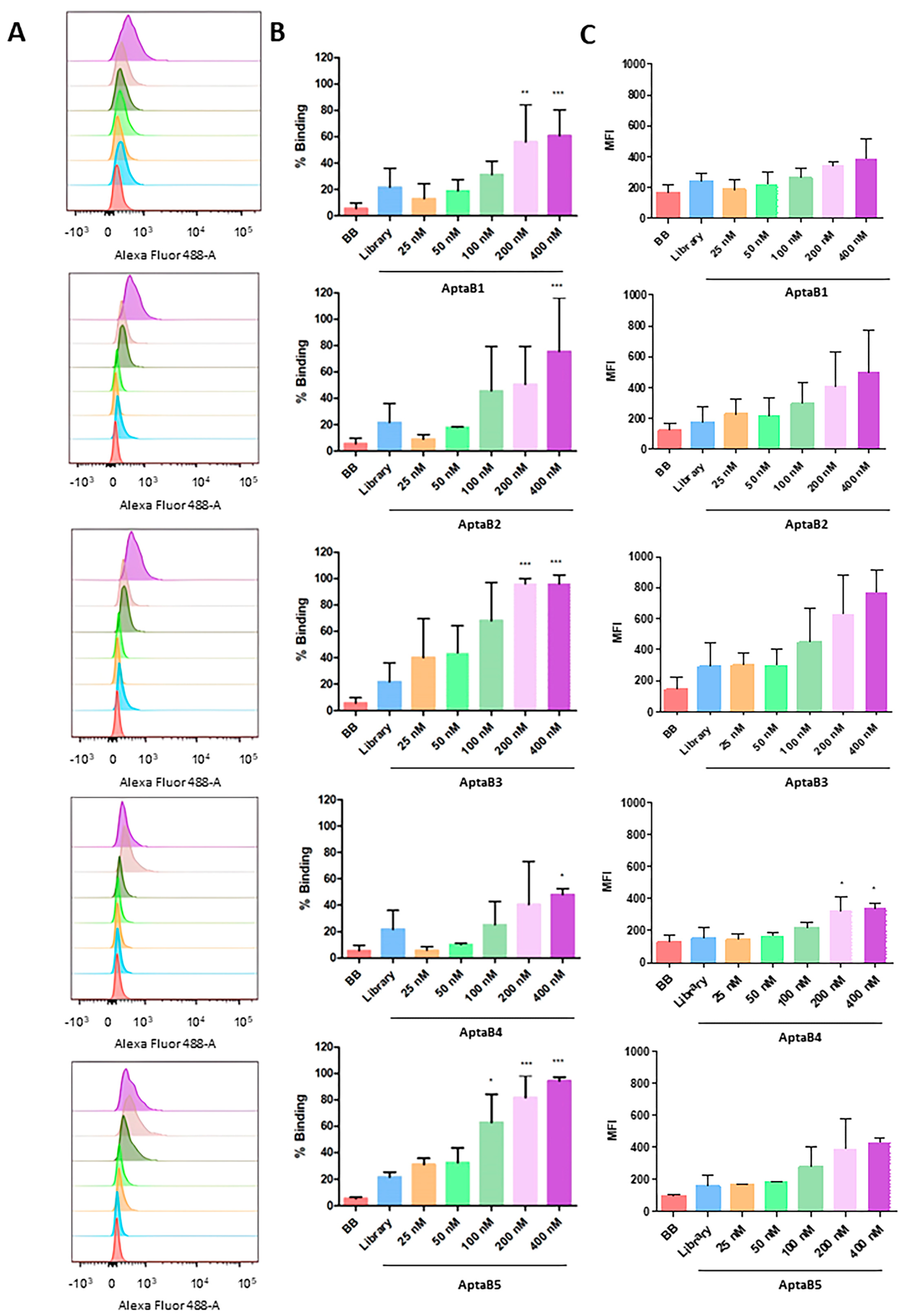
Figure 1.
Analysis of the binding capacity of the aptamer panel for the MDA-MB-231 strain. Histogram illustrating the percentage of cells incubated with binding buffer solution, initial library, and increasing doses of AptaB1–AptaB5 (A). Graphical representation of the mean percentage of binding of AptaB1–AptaB5 aptamers (B). Graphical representation of the average MFI (C). * p < 0.05, ** p < 0.01, *** p < 0.001.
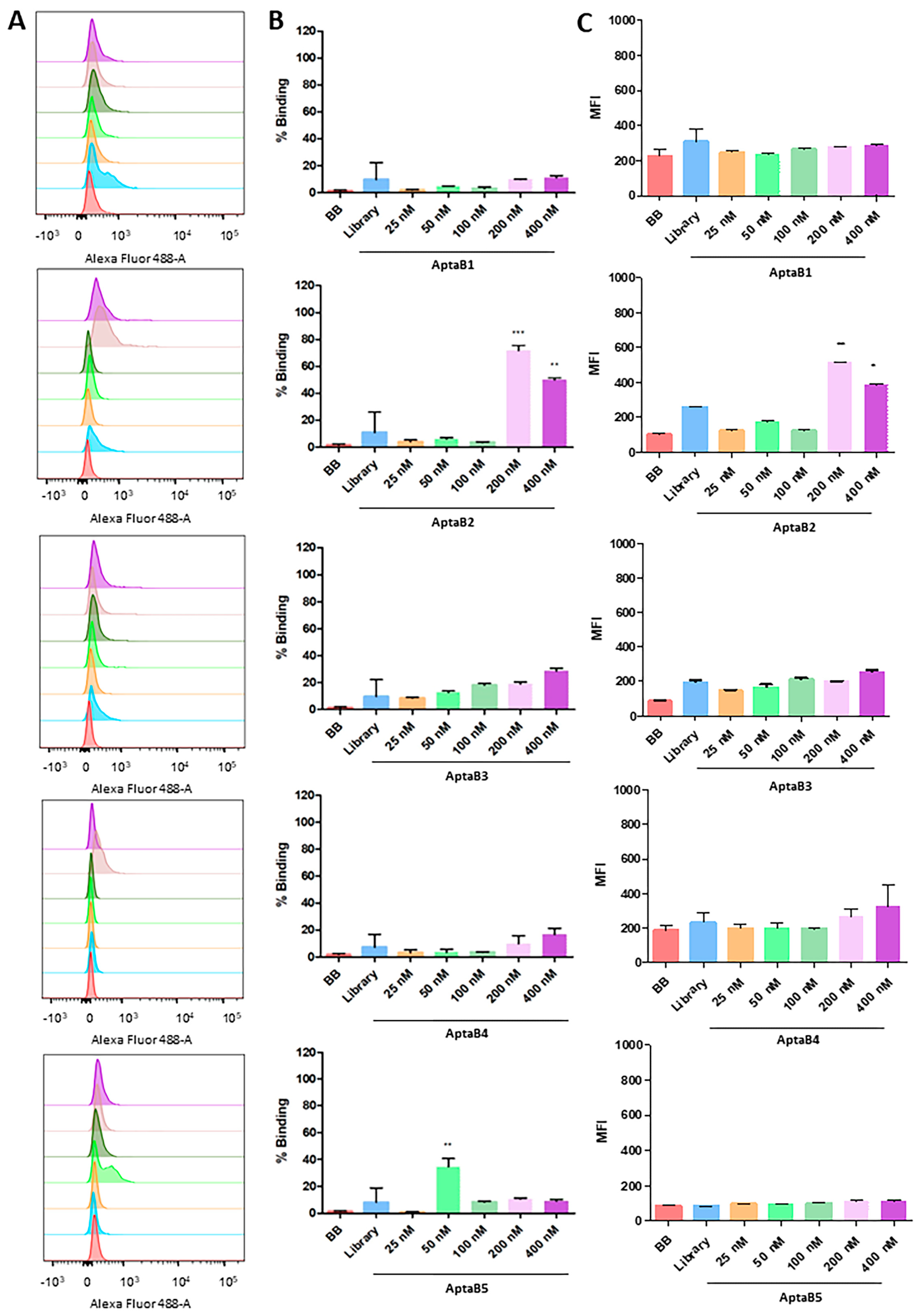
Figure 2.
Analysis of the recognition specificity of the aptamer panel for the non-tumor line MCF-10A. Histogram illustrating the percentage of cells incubated with binding buffer solution, initial library, and increasing doses of AptaB1–AptaB5 (A). Graphical representation of the mean percentage of binding of AptaB1–AptaB5 aptamers (B). Graphical representation of the average of MFI AptaB1–AptaB5 (C). * p < 0.05, ** p < 0.01, *** p < 0.001.
Figure 3.
Validation of the recognition and specificity of the aptamer panel. AptaB1-AptaB5 aptafluorescence (green) in MDA-MB-231 (A) and the absence of labeling in MCF-10A (B); nucleus labeled with DAPI (blue). Analysis and quantification of the localization of labeling observed in MDA-MB-231 (C).
Figure 4.
Aptafluorescence assay in a three-dimensional culture model. Core in blue (DAPI); aptamer conjugated to FAM in green. (A) Aptamer library, (B) AptaB1, (C) AptaB2, (D) AptaB3, (E) AptaB4, and (F) AptaB5. The images were obtained using imagexpress Micro Confocal equipment in a 10× objective. Bar = 200 µM.
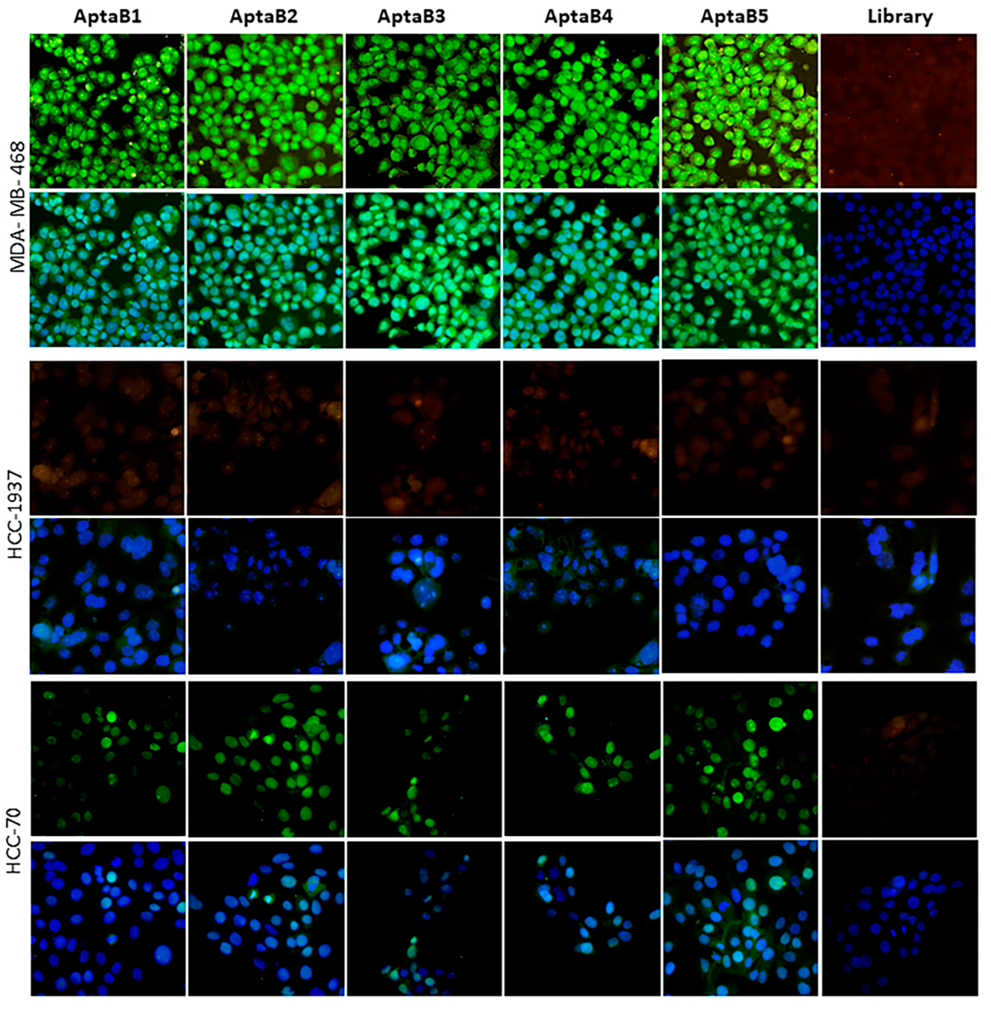
Figure 5.
Evaluation of the detection capacity of aptamers in triple-negative cell lines. Aptafluorescence assay with the aptamers AptaB1–AptaB5 or with the starting library—FAM (green) using triple-negative cell lines MDA-MB-468, HCC-70, and HCC-1937; nucleus stained with DAPI (blue).
Figure 5.
Evaluation of the detection capacity of aptamers in triple-negative cell lines. Aptafluorescence assay with the aptamers AptaB1–AptaB5 or with the starting library—FAM (green) using triple-negative cell lines MDA-MB-468, HCC-70, and HCC-1937; nucleus stained with DAPI (blue).
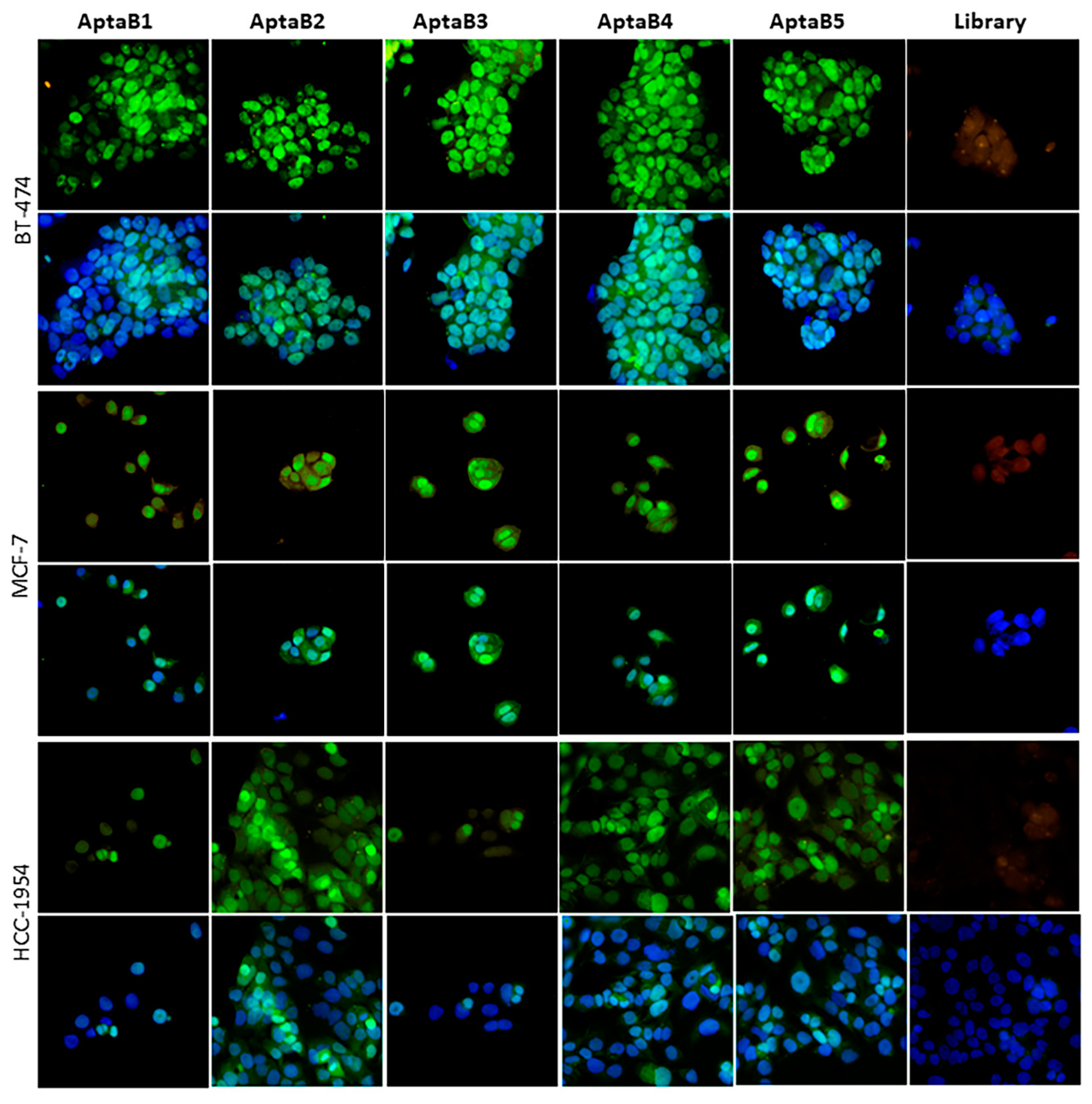
Figure 6.
Evaluation of the detection capacity of aptamers in cell lines of the luminal A, luminal B, and HER2+ molecular subtypes. Aptafluorescence assay with the aptamers AptaB1–AptaB5 or with the starting library—FAM (green) using MCF-7 (luminal A), BT-474 (luminal B), and HCC-1954 (HER2) cell lines; nucleus stained with DAPI (blue). Representative images of the library—FAM recognition. Overlay of the library—FAM recognition image and DAPI nucleus stain.
Figure 7.
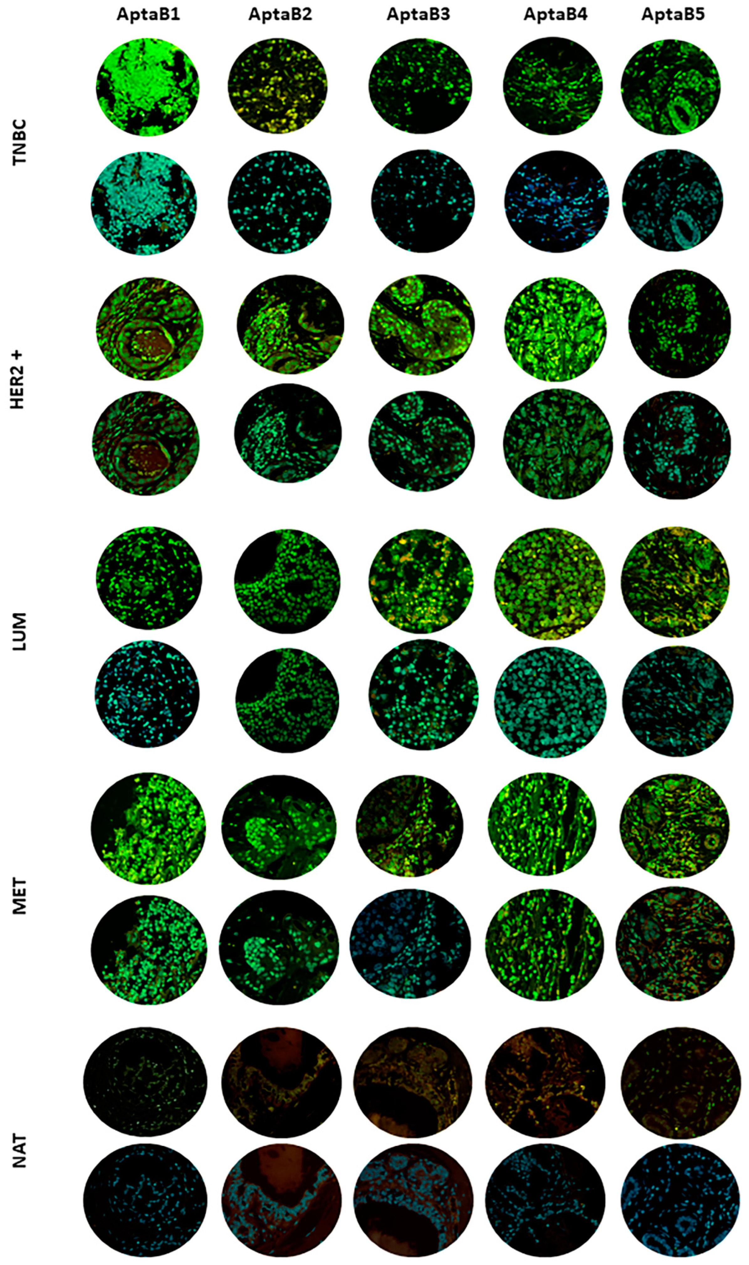
Validation of MD1–MD5 aptamer recognition in breast cancer samples using the tissue microarray technique (TMA). Triple-negative breast cancer (TNBC), HER2+ subtype (HER2+), luminal subtype (LUM), lymph node metastasis (MET), and adjacent normal tissue (NAT). Aptamers AptaB1–AptaB5 (green); cell nucleus stained with DAPI (blue).
Figure 7.
Validation of MD1–MD5 aptamer recognition in breast cancer samples using the tissue microarray technique (TMA). Triple-negative breast cancer (TNBC), HER2+ subtype (HER2+), luminal subtype (LUM), lymph node metastasis (MET), and adjacent normal tissue (NAT). Aptamers AptaB1–AptaB5 (green); cell nucleus stained with DAPI (blue).
Figure 8.
Representation of the secondary structure prediction of the aptamers selected for the MDA-MB-231 strain. The first column shows the results obtained with the NUPACK server and the second column shows the data from the mFold server. Below the structures, the free energy ΔG values are presented. For the structure obtained with NUPACK, the color of the dots is related to the equilibrium probability of paired bases, as showed in the equilibrium probability colored scale.
Figure 9.
Comparison of the predicted tertiary structures of aptamers obtained with RNAcompose with 2D structures predicted using the mFold and NUPACK servers. Aptamer models generated from mFold 2D structures are shown in blue, while models generated from NUPACK are shown in red. Structural alignment and calculation of TM scores were performed using the RNA-align server to quantitatively assess the similarity between the 3D models from the two sources. Tertiary structure visualizations were generated using Pymol.
Figure 10.
Analysis of conformational changes in structures during molecular dynamics simulation. The root mean square deviation (RMSD) is shown in Angstrons at the left, while the simulation time is given at the bottom. Black lines indicate the RMSD, while the shaded red line shows the tendency of the graph. (A): the RMSD of APTAB1 oscillated between 6 and 16 Å. The greatest variations happened between 30 ns and 300 ns. After 300 ns the RMSD stabilized around 13 Å and rose steadily until 16 Å. (B): The RMSD of AptaB2 did not stabilize throughout the simulation time. (C): AptaB3 was the less unstable aptamer among all 5. The RMSD of AptaB3 fluctuated around 14 Å and varied less than 4 Å for most of the simulation. (D): AptaB4 was quite unstable in the first half of the simulation, reaching 20 Å before the first 50 ns. Around 250 ns it stabilized near 24 Å and kept oscillating less than 4 Å until the end. (E): The RMSD of AptaB5 fluctuated around 13 Å, but showed great variations, reaching nearly 17 Å on its highest peak.
![Ijms 25 00840 g010]()
Figure 11.
Clusters analysis based on the change in RMSD. Each cluster represents a group of conformations assumed along the molecular dynamic trajectory with AptaB1–AptaB5. The five biggest clusters are shown for each aptamer. Time is given at the bottom, while the cluster index is given at the left. Each structure is shown as a square. Black horizontal bars indicate a high density of squares grouped. Red vertical lines delimit the simulation time of the three replicates. (A): The five biggest clusters of AptaB1. The most expressive cluster comprises the three replicates indicating only one representative structure for the whole simulation. (B): Among the five biggest clusters of AptaB2, the cluster 1 also comprises the three replicates and appears as the most significant in all of them. (C): Cluster 1 in also the most expressive cluster in all three replicates of AptaB3. However, in the first 200 ns cluster 2 and cluster 3 are more frequent than cluster 1. (D): Among the five biggest clusters of AptaB4, cluster 1 is the most frequent cluster in all three replicates. However, in the first 250 ns, the conformations are clustered in several other cluster in despite of cluster 1. (E): The five biggest clusters of AptaB5. The cluster 1 is more frequent in the replicates 1 and 3, however, in the simulation time between 500 ns and 100 ns (corresponding to replicate 2) the cluster 2 is the biggest cluster formed. This result indicates the existence of two stable conformations for this aptamer.
![Ijms 25 00840 g011]()
Figure 12.
The best binding complexes for potential aptamer targets. Image representing the best clusters from the molecular docking step for the TMPS3–AptaB1, CD151–AptaB2, TMEM205–AptaB3, CSKPAptaB4, TM9S3–AptaB5.1, and TM9S3–AptaB5.2 complexes. For the spatial orientation, the red portion indicates the extracellular region and the blue portion indicates the intracellular region.
Figure 13.
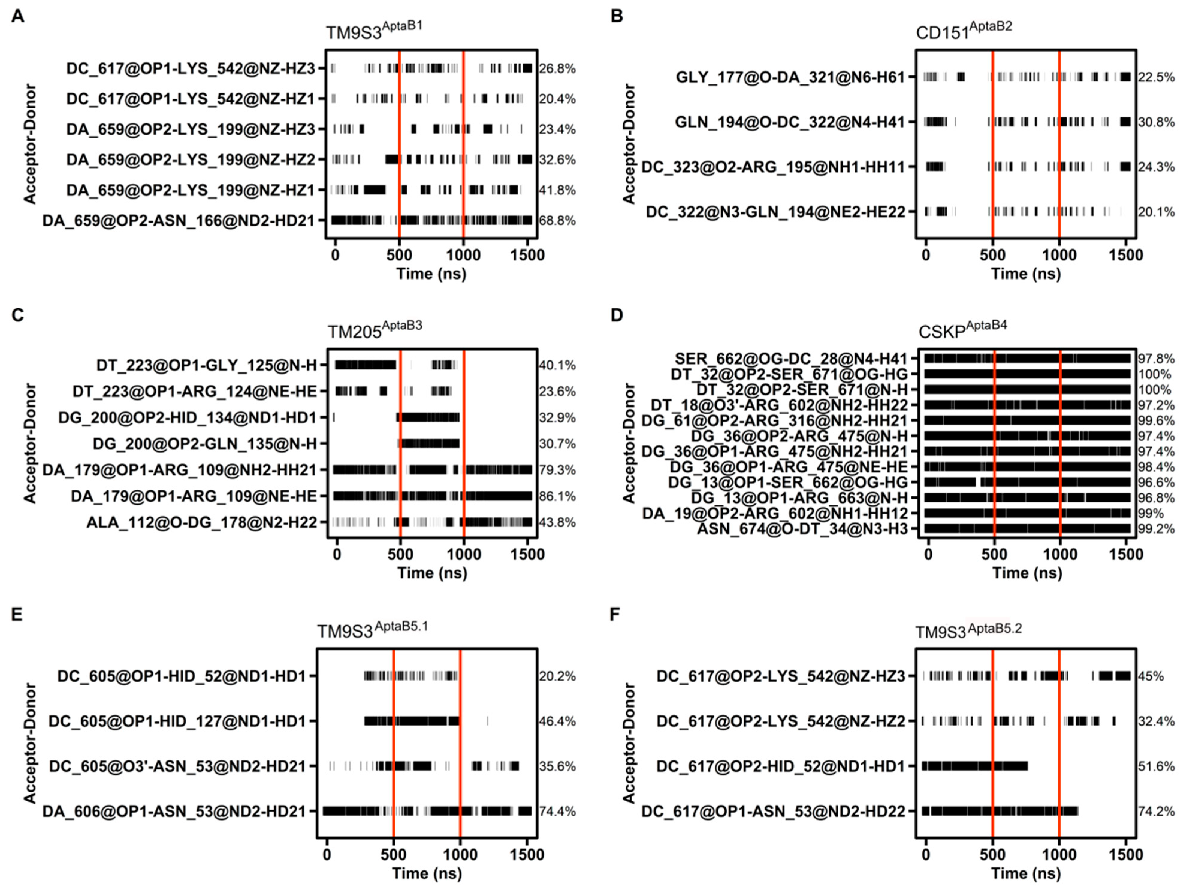
Hydrogen bond occupancy between the aptamer and the protein. The interacting pair of atoms are shown on the left, while the percentage of hbond occupancy is given on the right. The simulation time is shown in ns at the bottom. Horizontal black bars indicate each point of the simulation time that the interactions happened, whereas vertical red bars delimit each replicate time. Only hbond occupancies with 20% length or more are shown. (A): The binding of TM9S3 with AptaB1 is held mostly by the pair DA 659 and ASN 166. This interaction happens in all the replicates and covers 68.8% of the simulation time. 5 other weaker interactions above 20% hbond occupancy help to stabilize the binding throughout the simulation time. (B): In CD151AptaB2 there are just four interacting pairs with hbond occupancies over 20%, whereas the highest one happens for only 30.8% of the simulation. In several points of the simulation time there are no interaction happening at all. (C): In TM205AptaB3 There are 7 interacting pairs above 20% hbond occupancy. However, four of them does not happen in one of the replicates. (D): The system CSKPAptaB4 stands out in terms of hbond occupancy since its 12 higher hbond occupancy values are above 95%. (E): TM9S3AptaB5.1 formed 4 hbond with over 20% occupancy. Two of those hbonds does not happen in one of the replicates so the pair DA 606 and ASN 53 held the interaction for most of the time (74.4%). (F): similarly to TM9S3AptaB1, TM9S3AptaB5.2, also formed 4 hbond with over 20% occupancy and two of them also involved the same residues, ASN 53 and HID 52, being the former part of the most stable interacting pair (DC 617-ASN 53: 74.2%).
Figure 13.
Hydrogen bond occupancy between the aptamer and the protein. The interacting pair of atoms are shown on the left, while the percentage of hbond occupancy is given on the right. The simulation time is shown in ns at the bottom. Horizontal black bars indicate each point of the simulation time that the interactions happened, whereas vertical red bars delimit each replicate time. Only hbond occupancies with 20% length or more are shown. (A): The binding of TM9S3 with AptaB1 is held mostly by the pair DA 659 and ASN 166. This interaction happens in all the replicates and covers 68.8% of the simulation time. 5 other weaker interactions above 20% hbond occupancy help to stabilize the binding throughout the simulation time. (B): In CD151AptaB2 there are just four interacting pairs with hbond occupancies over 20%, whereas the highest one happens for only 30.8% of the simulation. In several points of the simulation time there are no interaction happening at all. (C): In TM205AptaB3 There are 7 interacting pairs above 20% hbond occupancy. However, four of them does not happen in one of the replicates. (D): The system CSKPAptaB4 stands out in terms of hbond occupancy since its 12 higher hbond occupancy values are above 95%. (E): TM9S3AptaB5.1 formed 4 hbond with over 20% occupancy. Two of those hbonds does not happen in one of the replicates so the pair DA 606 and ASN 53 held the interaction for most of the time (74.4%). (F): similarly to TM9S3AptaB1, TM9S3AptaB5.2, also formed 4 hbond with over 20% occupancy and two of them also involved the same residues, ASN 53 and HID 52, being the former part of the most stable interacting pair (DC 617-ASN 53: 74.2%).
![Ijms 25 00840 g013]()
Figure 14.
Decomposition of ΔGbind. The individual contribution of each residue to the total energy is depicted as vertical black bars. Negative energy values stand for residues working in favor of the binding process, while positive values denote residues disturbing the interaction. (A): Several residues are contributing to the binding of TM9S3 with AptaB1 reaching near 2.5 Kcal/mol. Contrastingly, highly positive energies are observed, particularly between residues 60 and 80. (B): Most of the residues in CD151 has nearly insignificant participation in the interaction with AptaB2. Despite showing some residues with highly negative energies, the number of residues repealing the ligand is superior, which resulted in the less negative ΔGbind observed among all the systems. (C): In TM205AptaB3 the number of negative energies overcomes the positive ones. Besides the residues with positive energies do not reach 1.5 kcal/mol. (D): The system CSKPAptaB4 has considerably more residues with negative energies than residues with positive energies. Besides, several residues are reaching −3 kcal/mol, while a few one’s overpass −4 kcal/mol. In contrast, the most positive energies do not reach 2 kcal/mol resulting in a deeply negative ΔGbind. (E): TM9S3AptaB5.1 has some similarities with TM9S3AptaB1. However, the negative contributions and positive ones have lower absolute values. (F): TM9S3AptaB5.2 is like TM9S3AptaB1, but with higher absolute values. The residues with the most negative energies in TM9S3AptaB5.2 reached −5 kcal/mol almost while in TM9S3AptaB5.1 the most negative energies are close to −2.5 kcal/mol.
![Ijms 25 00840 g014]()
Figure 15.
Summary schematic representation of Cell-SELEX (systematic evolution of ligands by exponential enrichment). 1—Initially, the DNA aptamer library (N30) was incubated with MDA-MB-231 target cells. 2—The cells were washed to remove unbounded sequences, and the bounded sequences were collected and amplified using PCR. 3—The aptamers went through the negative selection step in the MCF-10A cells, and the bound sequences were removed and eliminated, while the unbounded sequences were amplified using PCR and used in the subsequent Cell-SELEX rounds. 4—After 12 rounds of selection, the resulting aptamer pool was sequenced using the NGS methodology. 5—Finally, the aptamers were computationally analyzed, and the five most frequent sequences (AptaB1, AptaB2, AptaB3, AptaB4, and AptaB5) were selected for further validation steps.
Table 1.
Dissociation constant (Kd) analysis of aptamer binding to the target cell MDA-MB-231.
Table 1.
Dissociation constant (Kd) analysis of aptamer binding to the target cell MDA-MB-231.
| APTAMERS | KD VALUES |
|---|
| APTAB1 | 139 ± 14 nM |
| APTAB2 | 206 ± 41 nM |
| APTAB3 | 145 ± 31 nM |
| APTAB4 | 194 ± 0.7 nM |
| APTAB5 | 126 ± 19 nM |
Table 2.
Recognition of tissue samples from primary tumor, metastatic tissue, and tissue adjacent to the tumor.
Table 2.
Recognition of tissue samples from primary tumor, metastatic tissue, and tissue adjacent to the tumor.
| Aptamer | Sample | Recognition/
Total Number | % Recognition | Staining Intensity |
|---|
| AptaB1 | Adjacent tissue | 1/10 | 10% | (+) |
| Primary tumor tissue | 7/50 | 14% | (+++) |
| Metastatic tissue | 5/40 | 12.5% | (+++) |
| AptaB2 | Adjacent tissue | 1/10 | 10% | (+) |
| Primary tumor tissue | 18 /50 | 36% | (+++) |
| Metastatic tissue | 5/40 | 12.5% | (++) |
| AptaB3 | Adjacent tissue | 1/10 | 10% | (+) |
| Primary tumor tissue | 3/50 | 6% | (+++) |
| Metastatic tissue | 6/40 | 15% | (++) |
| AptaB4 | Adjacent tissue | 4/10 | 40% | (+) |
| Primary tumor tissue | 25/50 | 50% | (+++) |
| Metastatic tissue | 15/40 | 37.5% | (+++) |
| AptaB5 | Adjacent tissue | 3/10 | 30% | (+) |
| Primary tumor tissue | 20/50 | 40% | (+++) |
| Metastatic tissue | 27/40 | 67.5% | (+++) |
Table 3.
Recognition of breast carcinoma primary sites according to molecular subtype.
Table 3.
Recognition of breast carcinoma primary sites according to molecular subtype.
| Aptamer | Molecular Subtype
from Primary Tumor | Recognition/
Total Number | % Recognition | Staining Intensity |
|---|
| AptaB1 | Luminal | 3/28 | 10.7 | (+++) |
| HER 2 | 3/7 | 42 | (+++) |
| Triple-negative | 1/10 | 10 | (+++) |
| AptaB2 | Luminal | 8/28 | 28 | (+++) |
| HER 2 | 5/7 | 70 | (+++) |
| Triple-negative | 4/10 | 40 | (+++) |
| AptaB3 | Luminal | 1/28 | 3.5 | (+++) |
| HER 2 | 1/7 | 14 | (+++) |
| Triple-negative | 1/10 | 10 | (++) |
| AptaB4 | Luminal | 12/28 | 42 | (+++) |
| HER 2 | 6/7 | 85 | (+++) |
| Triple-negative | 4/10 | 40 | (++) |
| AptaB5 | Luminal | 9/28 | 32 | (+++) |
| HER 2 | 5/7 | 70 | (+++) |
| Triple-negative | 5/10 | 50 | (+++) |
Table 4.
Recognition of metastatic lymph node tissue samples according to molecular subtype.
Table 4.
Recognition of metastatic lymph node tissue samples according to molecular subtype.
| Aptamer | Molecular Subtype of the
Metastatic Sample | Recognition/Number of Samples | % Recognition | Staining Intensity |
|---|
| AptaB1 | Luminal | 3/14 | 21% | (+++) |
| HER 2 | 0/9 | - | (−) |
| Triple-negative | 0/8 | - | (−) |
| AptaB2 | Luminal | 1/14 | 7.1% | (+++) |
| HER 2 | 2/9 | 22% | (+++) |
| Triple-negative | 2/8 | 25% | (+++) |
| AptaB3 | Luminal | 1/14 | 3.5% | (+++) |
| HER 2 | 1/9 | 11% | (+++) |
| Triple-negative | 3/8 | 37.5% | (++) |
| AptaB4 | Luminal | 6/14 | 42% | (+++) |
| HER 2 | 1/9 | 11% | (+++) |
| Triple-negative | 5/8 | 62% | (++) |
| AptaB5 | Luminal | 10/14 | 32% | (+++) |
| HER 2 | 7/9 | 77% | (+++) |
| Triple-negative | 5/8 | 62% | (+++) |
Table 5.
Recognition of aptamers according to the degree of tumor staging.
Table 5.
Recognition of aptamers according to the degree of tumor staging.
| Stage | Number of Samples | AptaB1 | AptaB2 | AptaB3 | AptaB4 | AptaB5 |
|---|
| I | 4 | 0 | 1 | 0 | 3 | 2 |
| II | 39 | 4 | 15 | 3 | 20 | 4 |
| III | 3 | 2 | 1 | 1 | 2 | 3 |
Table 6.
Recognition of aptamers according to the histological grade of the tumor.
Table 6.
Recognition of aptamers according to the histological grade of the tumor.
| Grade | Number of Samples | AptaB1 | AptaB2 | AptaB3 | AptaB4 | AptaB5 |
|---|
| I | 8 | 1 | 4 | 0 | 5 | 1 |
| II | 29 | 4 | 10 | 3 | 17 | 11 |
| III | 9 | 1 | 4 | 0 | 4 | 5 |
Table 7.
Recognition of clinical samples by aptamers according to the TMN classification.
Table 7.
Recognition of clinical samples by aptamers according to the TMN classification.
| TNM | Number of Samples | AptaB1 | AptaB2 | AptaB3 | AptaB4 | AptaB5 |
|---|
| T1N0M0 | 4 | 0 | 1 | 0 | 3 | 2 |
| T2N0M0 | 29 | 4 | 11 | 2 | 15 | 10 |
| T2N1M0 | 6 | 0 | 2 | 1 | 3 | 3 |
| T2N3M0 | 1 | 1 | 0 | 1 | 0 | 1 |
| T3N0M0 | 4 | 0 | 2 | 0 | 2 | 0 |
| T3N1M0 | 1 | 0 | 0 | 0 | 1 | 1 |
| T4N0M0 | 3 | 1 | 2 | 0 | 2 | 2 |
| T4N1M0 | 2 | 1 | 1 | 0 | 1 | 2 |
Table 8.
Diagnostic index calculated from the recognition of aptamers in primary, metastatic, and adjacent tumor tissue.
Table 8.
Diagnostic index calculated from the recognition of aptamers in primary, metastatic, and adjacent tumor tissue.
| Aptamers | Sensitivity | Specificity | Accuracy |
|---|
| AptaB1 | 13% | 90% | 21% |
| AptaB2 | 26% | 90% | 32% |
| AptaB3 | 10% | 90% | 18% |
| AptaB4 | 44% | 60% | 46% |
| AptaB5 | 52% | 70% | 54% |
| AptaB4 + AptaB5 | 77% | 40% | 73% |
| AptaB2 + AptaB4 + AptaB5 | 87% | 30% | 81% |
| AptaB2 + AptaB3 + AptaB4 + AptaB5 | 89% | 30% | 83% |
| AptaB1 + AptaB2 + AptaB3 + AptaB4 + AptaB5 | 96% | 30% | 89% |
Table 9.
Haddock score for the result of the molecular docking with the selected proteins and representative structures of the AptaB1, AptaB2, AptaB3, AptaB4, AptaB5.1, and AptaB5.2 aptamers.
Table 9.
Haddock score for the result of the molecular docking with the selected proteins and representative structures of the AptaB1, AptaB2, AptaB3, AptaB4, AptaB5.1, and AptaB5.2 aptamers.
| | Protein–AptaB1 | Haddock Score |
|---|
| A | CSKP–AptaB1 | −34.9 +/− 7.5 |
| B | TM9S3–AptaB1 | −76.7 +/− 33.4 |
| C | TMEM205–AptaB1 | −48.1 +/− 8.0 |
| D | CD151–AptaB1 | 2.8 +/− 9.4 |
| | Protein–AptaB2 | Haddock Score |
| A | CSKP–AptaB2 | −8.3 +/− 8.9 |
| B | TM9S3–AptaB2 | −11.1 +/− 18.0 |
| C | TMEM205–AptaB2 | −46.7 +/− 6.1 |
| D | CD151–AptaB2 | −53.1 +/− 9.2 |
| | Protein–AptaB3 | Haddock Score |
| A | CSKP–AptaB3 | −8.7 +/− 21.7 |
| B | TM9S3–AptaB3 | −31.2 +/− 3.9 |
| C | TMEM205–AptaB3 | −34.2 +/− 3.5 |
| D | CD151–AptaB3 | 17.3 +/− 9.9 |
| | Protein–AptaB4 | Haddock Score |
| A | CSK–AptaB4 | −34.7 +/− 11.1 |
| B | TM9S3–AptaB4 | −22.3 +/− 4.0 |
| C | TMEM205–AptaB4 | −23.9 +/− 6.5 |
| D | CD151–AptaB4 | −8.4 +/− 25.8 |
| | Protein–AptaB5.1 | Haddock Score |
| A | CSKP–AptaB5.1 | 20.5 +/− 27.0 |
| B | TM9S3–AptaB5.1 | −41.2 +/− 16.2 |
| C | TMEM205–AptaB5.1 | 12.3 +/− 11.5 |
| D | CD151–AptaB5.1 | 18.0 +/− 13.2 |
| | Protein–AptaB5.2 | Haddock Score |
| A | CSKP–AptaB5.2 | −4.7 +/− 22.0 |
| B | TM9S3–AptaB5.2 | −81.2 +/− 4.4 |
| C | TMEM205–AptaB5.2 | −3.7 +/− 13.9 |
| D | CD151–AptaB5.2 | 6.5 +/− 6.5 |
Table 10.
Binding free energy change (ΔGbind) for all complexes calculated using MM/GBSA.
Table 10.
Binding free energy change (ΔGbind) for all complexes calculated using MM/GBSA.
| System | ΔEvdw | Δele | Δegb | ΔGesurf | ΔGbind |
|---|
| TM9S3AptaB1 | −212.04 | 4821.73 | −4654.34 | −23.45 | −68.1 ± 2.7 |
| CD151AptaB2 | −31.49 | 983.92 | −952.11 | −3.99 | −03.6 ± 3.7 |
| TM205AptaB3 | −52.77 | 874.05 | −842.43 | −13.90 | −35.0 ± 3.3 |
| CSKPAptaB4 | −246.40 | 5174.56 | −5015.07 | −30.90 | −117.8 ± 2.2 |
| TMS9AptaB 5.1 | −209.31 | 4883.27 | −4703.32 | −24.24 | −53.6 ± 2.1 |
| TMS9AptaB 5.2 | −210.58 | 4925.62 | −4745.78 | −28.66 | −59.4 ± 2.5 |

 ,
, 


