Angular Rate Optimal Design for the Rotary Strapdown Inertial Navigation System

Abstract

Due to the characteristics of high precision for a long duration, the rotary strapdown inertial navigation system (RSINS) has been widely used in submarines and surface ships. Nowadays, the core technology, the rotating scheme, has been studied by numerous researchers. It is well known that as one of the key technologies, the rotating angular rate seriously influences the effectiveness of the error modulating. In order to design the optimal rotating angular rate of the RSINS, the relationship between the rotating angular rate and the velocity error of the RSINS was analyzed in detail based on the Laplace transform and the inverse Laplace transform in this paper. The analysis results showed that the velocity error of the RSINS depends on not only the sensor error, but also the rotating angular rate. In order to minimize the velocity error, the rotating angular rate of the RSINS should match the sensor error. One optimal design method for the rotating rate of the RSINS was also proposed in this paper. Simulation and experimental results verified the validity and superiority of this optimal design method for the rotating rate of the RSINS.

1. Introduction

The operation of an inertial navigation system (INS) depends on Newton' second law [1]. The inertial navigation is the process whereby the measurements of inertial sensors (gyroscopes and accelerometers) calculate the position and velocity of the vehicle. Unlike other types of navigation systems, the INS is an entirely independent navigation system, since it is not dependent on the transmission of signals from the vehicle or reception from an external source. However, the fatal flaw of the INS is that the navigation error caused by the bias of the inertial sensors increases with time. Therefore, the precision of the INS is subject to the precision of inertial sensors [2,3].

For the original INS, the inertial sensors are mounted on a stable platform, which is mechanically isolated from the rotational motion of the vehicle [4]. Due to the mechanical complexity of the platform system, a new type of INS, which is called the strapdown inertial navigation system (SINS), is replacing the traditional platform inertial navigation system. The SINS has the advantages of lower cost, smaller size and greater reliability compared with platform systems, since the inertial sensors are attached rigidly to the body of the vehicle [5].

Since the navigation error caused by the bias of the inertial sensors increases with time, researchers proposed the rotation modulation method to reduce the impact on the SINS, which is installed on the vehicle through the turntable. The rotation modulation method modulates the bias of inertial sensors into a zero-mean and periodical form to inhibit the error propagation, and then, the localization precision of the SINS will be enhanced effectively. This kind of rotary strapdown inertial navigation system (RSINS) has been applied by the U.S. Navy since the 1960s [6-8]. However, the disadvantage of the rotation modulation is that it cannot modulate the installation error and the symmetric scale factor error of the inertial sensors, but it also produces instantaneous velocity error [8-10]. As a result, the design of the rotating angular rate has became a hotspot of rotation modulation.

The RSINS accuracy influenced by the non-uniform rotation angular rate is analyzed by Dr. Che [11]. The rotating scheme design method of the non-uniform rotating angular rate is proposed in [12]. However, until now, no one has been able to figure out an effective optimal rotating angular rate design method of the RSINS in theory. Therefore, in this article, a novel rotating angular rate design discipline, which will fill the gap, was proposed. We focused on the optimal design of the rotating angular rate utilizing the Laplace transform and the inverse Laplace transform in this article, and this paper is organized as follows. In Section 2, the principle of the rotation modulation and the inertial sensor error model are introduced. The design method of the rotating angular rate is proposed in Section 3. Simulations and experiments are carried out in Section 4 and 5, respectively, to verify the correctness of the design method.

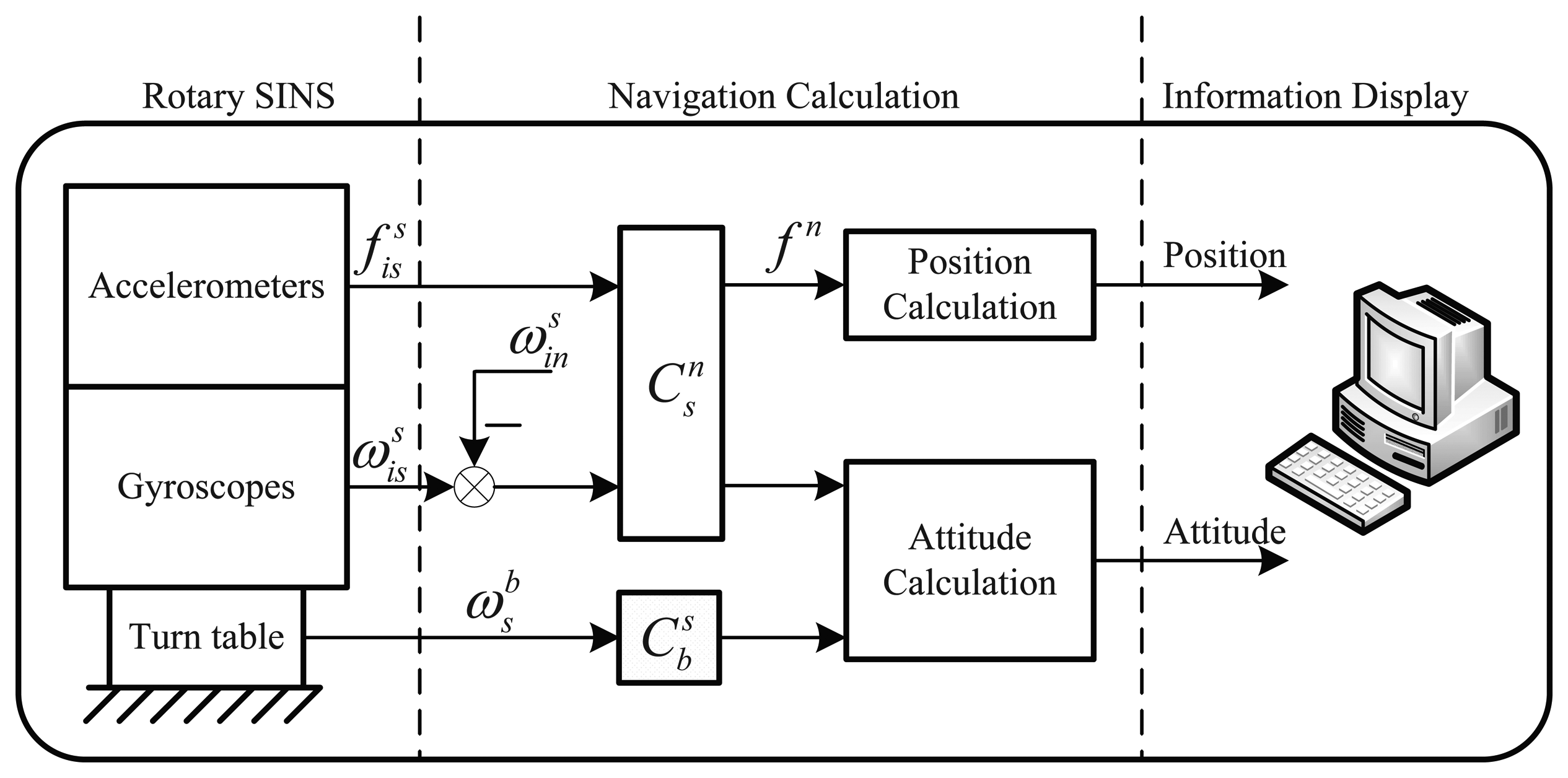
2. Principle of the Rotation Modulation and the Error Model

2.1. Rotary Strapdown Inertial Navigation System

As the SINS is installed on the vehicle through the turntable, the structure of the RSINS, which is shown as Figure 1, is different from the SINS. Since the middle of the last century, rotation modulation has been widely applied to the SINS [9,10].

Classified by the number of the rotating axes, the RSINS can be divided into single-axis RSINS and the dual-axis RSINS [13]. However, the purpose is the same, i.e. to compensate for the effect of inertial sensor errors without external information [14].

Additionally, we must say that any technique has its limitations, and rotation modulation is no exception. One fatal shortcoming of rotation modulation is that it will produce instantaneous velocity error that cannot be ignored during the rotating period, and the error exists in any rotating mode [8,15].

The essence of rotation modulation is the error self-compensation [16-18]. It modulates the inertial sensor errors in terms of periodical rotation. It is an effective method to enhance the navigation accuracy under low-accuracy sensors conditions [19-21]. The inertial sensor errors neither disappear nor change, but offset during the whole rotation period [21-24].

As the inertial measurement unit (IMU) connects with the vehicle indirectly through the turntable, a new frame, the sensor frame (s frame), is introduced in the RSINS. It is supposed that the body frame (b frame) and the navigation frame (n frame) are coherent. This means $C_n^b=I$ and $C_b^s=C_n^s$. The output of the inertial sensors is transformed from the s frame to the n frame by a direction cosine matrix. Suppose the s frame and n frame overlap at the initial time, and the IMU is controlled to rotate uniformly at a certain speed, ω_r, along the vertical direction. The direction cosine matrix from the s frame to the n frame can be expressed by:

$$C_s^n={(C_n^s)}^T={(C_b^s)}^T=\left[\begin{array}{ccc}cos{\omega }_{r}t& -sin{\omega }_{r}t& 0\\ sin{\omega }_{r}t& cos{\omega }_{r}t& 0\\ 0& 0& 1\end{array}\right]$$

(1)

The modulated constant bias of the gyroscope in the n frame [ɛ _E1 ɛ_N1 ɛ_U1]^T can be described by the following equation.

$$\left[\begin{array}{c}{\mathit{\varepsilon }}_{E1}\\ {\mathit{\varepsilon }}_{N1}\\ {\mathit{\varepsilon }}_{U1}\end{array}\right]=C_s^n\left[\begin{array}{c}{\mathit{\varepsilon }}_{x0}\\ {\mathit{\varepsilon }}_{y0}\\ {\mathit{\varepsilon }}_{z0}\end{array}\right]=\left[\begin{array}{c}{\mathit{\varepsilon }}_{x0}cos{\omega }_{r}t-{\mathit{\varepsilon }}_{y0}sin{\omega }_{r}t\\ {\mathit{\varepsilon }}_{x0}sin{\omega }_{r}t+{\mathit{\varepsilon }}_{y0}cos{\omega }_{r}t\\ {\mathit{\varepsilon }}_{z0}\end{array}\right]$$

(2)

where ɛ_x0, ɛ_y0, ɛ_z0 denote the constant bias of the three orthogonal gyroscopes. From Equation (2), it is obviously known that the horizontal constant bias of the gyroscope can be modulated into periodic and zero-mean signals by periodically rotating the IMU. Analogously, it has the same result for the accelerometer. This technique can be utilized to modulate the inertial sensor error, which is vertical to the rotating axis, in order to enhance the positioning accuracy of the RSINS.

2.2. The Sensor Error Model of the RSINS

The inertial sensor error mainly includes the constant bias, the scale factor error and the installation error of the optical gyroscope and the constant bias of the accelerometer. In Section 2, we will focus on the relationship between the inertial sensor error and the performance of the RSINS.

2.2.1. Constant Bias of Optical Gyroscopes and Accelerometers

The modulated constant bias of the gyroscope and the accelerometer in the n frame can be described by Equations (2) and (3), respectively.

$$\left[\begin{array}{c}{\nabla }_E\\ {\nabla }_N\end{array}\right]=\left[\begin{array}{cc}cos{\omega }_{r}t& -sin{\omega }_{r}t\\ sin{\omega }_{r}t& cos{\omega }_{r}t\end{array}\right]\left[\begin{array}{c}{\nabla }_{x0}\\ {\nabla }_{y0}\end{array}\right]=\left[\begin{array}{c}{\nabla }_{x0}cos{\omega }_{r}t-{\nabla }_{y0}sin{\omega }_{r}t\\ {\nabla }_{y0}sin{\omega }_{r}t+{\nabla }_{x0}cos{\omega }_{r}t\end{array}\right]$$

(3)

where ∇_x0 and ∇_y0 are the constant bias of horizontal accelerometers.

2.2.2. Scale Factor Error of Optical Gyroscopes

The equivalent bias of gyroscopes, ε′, caused by the scale factor asymmetric error of gyroscopes can be described by:

$$\left[\begin{array}{c}{{\mathit{\varepsilon }}_x}^{\prime }\\ {{\mathit{\varepsilon }}_y}^{\prime }\\ {{\mathit{\varepsilon }}_z}^{\prime }\end{array}\right]=\left[\begin{array}{ccc}{K}_{gx}& 0& 0\\ 0& K_{gy}& 0\\ 0& 0& K_{gz}\end{array}\right]\left[\begin{array}{c}{\omega }_x\\ {\omega }_y\\ {\omega }_z\end{array}\right]=\left[\begin{array}{c}{K}_{gx}\cdot {\omega }_{ie}\cdot cosL\cdot sin{\omega }_{r}t\\ K_{gy}\cdot {\omega }_{ie}\cdot cosL\cdot cos{\omega }_{r}t\\ K_{gz}({\omega }_{ie}\cdot sinL+{\omega }_r)\end{array}\right]$$

(4)

where K_gx, K_gy and K_gz denote the scale factor asymmetry errors of gyroscopes along the x, y and z axes, respectively; ω_ie denotes the Earth's rotation rate; L denotes the local latitude; [ω_x ω_y ω_z]^T denotes the output of gyroscopes, and its theoretical value is:

$$\left[\begin{array}{c}{\omega }_x\\ {\omega }_y\\ {\omega }_z\end{array}\right]=\left[\begin{array}{c}{\omega }_{ie}\cdot cosL\cdot sin{\omega }_{r}t\\ {\omega }_{ie}\cdot cosL\cdot cos{\omega }_{r}t\\ {\omega }_{ie}\cdot sinL+{\omega }_r\end{array}\right]$$

(5)

Therefore, the modulated equivalent bias of gyroscopes, ε′′, in the n frame can be described by:

$$\left[\begin{array}{c}{\mathit{\varepsilon }}_{E2}\\ {\mathit{\varepsilon }}_{N2}\\ {\mathit{\varepsilon }}_{U2}\end{array}\right]=\left[\begin{array}{ccc}cos{\omega }_{r}t& -sin{\omega }_{r}t& 0\\ sin{\omega }_{r}t& cos{\omega }_{r}t& 0\\ 0& 0& 1\end{array}\right]\left[\begin{array}{c}{{\mathit{\varepsilon }}_x}^{\prime }\\ {{\mathit{\varepsilon }}_y}^{\prime }\\ {{\mathit{\varepsilon }}_z}^{\prime }\end{array}\right]=\left[\begin{array}{c}{{\mathit{\varepsilon }}_x}^{\prime }cos{\omega }_{r}t-{{\mathit{\varepsilon }}_y}^{\prime }sin{\omega }_{r}t\\ {{\mathit{\varepsilon }}_y}^{\prime }cos{\omega }_{r}t-{{\mathit{\varepsilon }}_x}^{\prime }sin{\omega }_{r}t\\ {{\mathit{\varepsilon }}_z}^{\prime }\end{array}\right]$$

(6)

2.2.3. Installation Error of Optical Gyroscopes

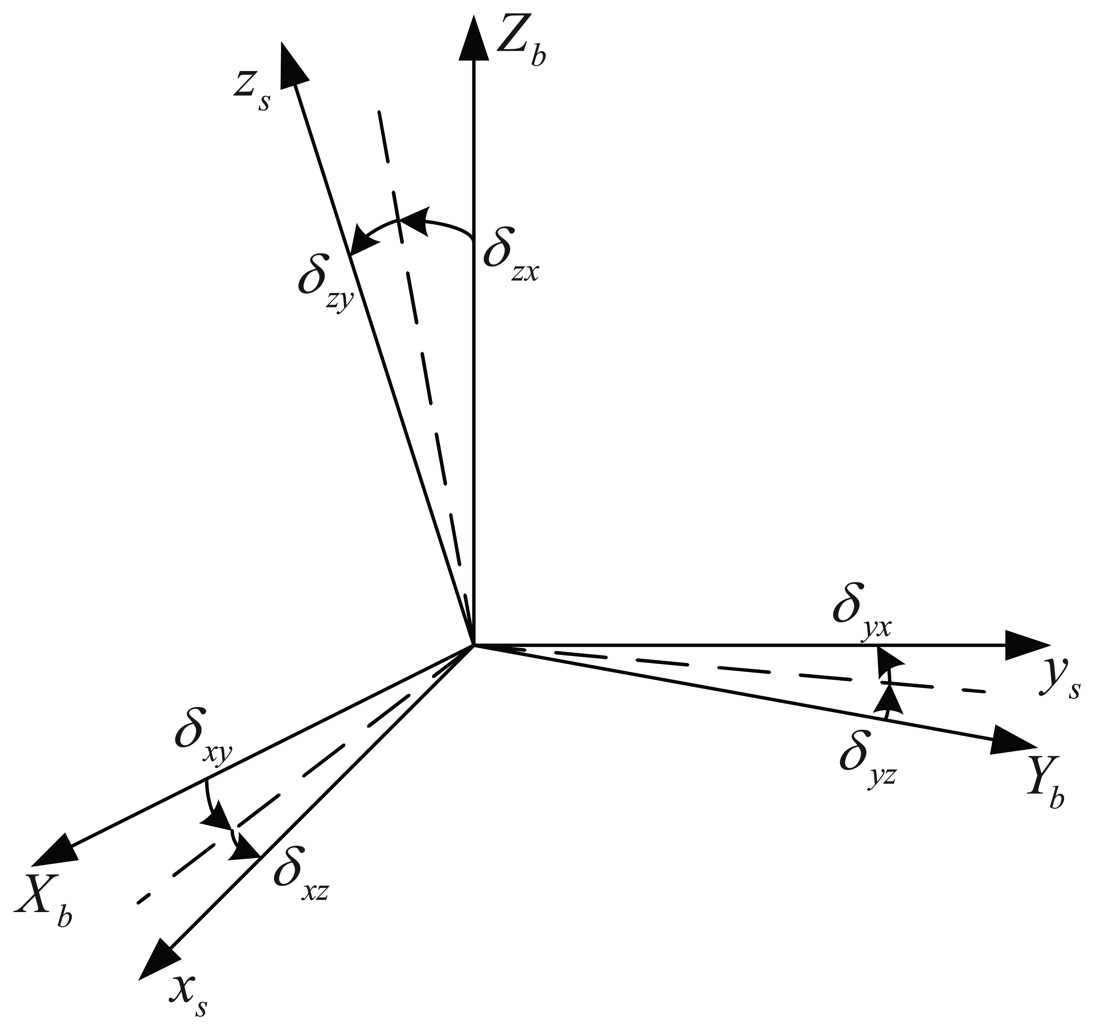
The inertial sensors should be installed orthogonally in theory. However, the actually s frame is not orthogonal and cannot coincide with the b frame, as shown in Figure 2. The small-angle δ_ij is defined as the installation error between the i axis of the s frame and the j axis of the b frame. Therefore, the installation error matrix can be described as:

$$\mathrm{\Delta }{C}_b^s=\left[\begin{array}{ccc}0& -{\delta }_{xz}& {\delta }_{xy}\\ {\delta }_{yz}& 0& -{\delta }_{yx}\\ -{\delta }_{yz}& {\delta }_{zx}& 0\end{array}\right]$$

(7)

The equivalent bias of gyroscopes, ${\mathit{\varepsilon }}_z^{″}$, caused by the installation error can be described by:

$$\begin{array}{cc}\left[\begin{array}{c}{\mathit{\varepsilon }}_x^{″}\\ {\mathit{\varepsilon }}_y^{″}\\ {\mathit{\varepsilon }}_z^{″}\end{array}\right]& =\left[\begin{array}{ccc}0& -{\delta }_{xz}& {\delta }_{xy}\\ {\delta }_{yz}& 0& -{\delta }_{yx}\\ -{\delta }_{yz}& {\delta }_{zx}& 0\end{array}\right]\left[\begin{array}{c}{\omega }_x\\ {\omega }_y\\ {\omega }_z\end{array}\right]\hfill \\ & =\left[\begin{array}{c}{\delta }_{xy}({\omega }_{ie}sinL+{\omega }_r)-{\delta }_{xz}{\omega }_{ie}cosLcos{\omega }_{r}t\\ -{\delta }_{yx}({\omega }_{ie}sinL+{\omega }_r)+{\delta }_{yz}{\omega }_{ie}cosLsin{\omega }_{r}t\\ {\delta }_{zx}{\omega }_{ie}cosLcos{\omega }_{r}t-{\delta }_{yz}{\omega }_{ie}cosLsin{\omega }_{r}t\end{array}\right]\end{array}$$

(8)

Therefore, the modulated equivalent bias of gyroscopes, ε″, in the n frame can be described by:

$$\left[\begin{array}{c}{\mathit{\varepsilon }}_{E3}\\ {\mathit{\varepsilon }}_{N3}\\ {\mathit{\varepsilon }}_{U3}\end{array}\right]=\left[\begin{array}{ccc}cos{\omega }_{r}t& -sin{\omega }_{r}t& 0\\ sin{\omega }_{r}t& cos{\omega }_{r}t& 0\\ 0& 0& 1\end{array}\right]\left[\begin{array}{c}{{\mathit{\varepsilon }}_x}^{″}\\ {{\mathit{\varepsilon }}_y}^{″}\\ {{\mathit{\varepsilon }}_z}^{″}\end{array}\right]=\left[\begin{array}{c}{{\mathit{\varepsilon }}_x}^{″}cos{\omega }_{r}t-{{\mathit{\varepsilon }}_y}^{″}sin{\omega }_{r}t\\ {{\mathit{\varepsilon }}_y}^{″}cos{\omega }_{r}t+{{\mathit{\varepsilon }}_x}^{″}sin{\omega }_{r}t\\ {{\mathit{\varepsilon }}_z}^{″}\end{array}\right]$$

(9)

2.2.4. Error Model of Inertial Sensors in the RSINS

Concerning the study above, the error model of the RSINS can be described as

$$\left[\begin{array}{c}{\nabla }_E\\ {\nabla }_N\\ 0\\ {\mathit{\varepsilon }}_E\\ {\mathit{\varepsilon }}_N\\ {\mathit{\varepsilon }}_U\end{array}\right]=\left[\begin{array}{c}{\nabla }_E\\ {\nabla }_N\\ 0\\ {\mathit{\varepsilon }}_{E1}+{\mathit{\varepsilon }}_{E2}+{\mathit{\varepsilon }}_{E3}\\ {\mathit{\varepsilon }}_{N1}+{\mathit{\varepsilon }}_{N2}+{\mathit{\varepsilon }}_{N3}\\ {\mathit{\varepsilon }}_{U1}+{\mathit{\varepsilon }}_{U2}+{\mathit{\varepsilon }}_{U3}\end{array}\right]=W_1(t)+W_2(t)+W_3(t)$$

(10)

where W₁(t), W₂(t) and W₃(t) represent the constant bias error of inertial sensors, the scale factor error and the installation error of gyroscopes, respectively.

$$\begin{array}{cc}{W}_1(t)=\left[\begin{array}{c}{\nabla }_{x0}cos{\omega }_{r}t-{\nabla }_{y0}sin{\omega }_{r}t\\ {\nabla }_{x0}sin{\omega }_{r}t+{\nabla }_{y0}cos{\omega }_{r}t\\ 0\\ {\mathit{\varepsilon }}_{x0}cos{\omega }_{r}t-{\mathit{\varepsilon }}_{y0}sin{\omega }_{r}t\\ {\mathit{\varepsilon }}_{y0}cos{\omega }_{r}t+{\mathit{\varepsilon }}_{x0}sin{\omega }_{r}t\\ {\mathit{\varepsilon }}_{z0}\end{array}\right],& W_2(t)=\left[\begin{array}{c}0\\ 0\\ 0\\ {\mathit{\varepsilon }}_x^{\prime }cos{\omega }_{r}t-{\mathit{\varepsilon }}_y^{\prime }sin{\omega }_{r}t\\ {\mathit{\varepsilon }}_y^{\prime }cos{\omega }_{r}t+{\mathit{\varepsilon }}_x^{\prime }sin{\omega }_{r}t\\ {\mathit{\varepsilon }}_z^{\prime }\end{array}\right],\\ W_3(t)=\left[\begin{array}{c}0\\ 0\\ 0\\ {\mathit{\varepsilon }}_x^{″}cos{\omega }_{r}t-{\mathit{\varepsilon }}_y^{″}sin{\omega }_{r}t\\ {\mathit{\varepsilon }}_y^{″}cos{\omega }_{r}t-{\mathit{\varepsilon }}_x^{″}sin{\omega }_{r}t\\ {\mathit{\varepsilon }}_z^{″}\end{array}\right]\end{array}$$

It can be seen from Equation (10) that the error model of the RSINS is a function that depends on not only the error of inertial sensors, but also the rotating angular rate. Therefore, the performance of the RSINS will be influenced by the rotating angular rate.

3. Optimal Design Method for the Rotating Angular Rate in the RSINS

The previous analysis shows that the error model of the RSINS bears on both the inertial sensor error and the rotating angular rate. Therefore, this section will investigate the relationship between the rotating angular rate and the RSINS performance.

3.1. The Velocity Error Equation of the RSINS

Based on the spherical Earth model, ignoring the movement of the vehicle, suppose the IMU rotates along the vertical axis at ω_r; the error model of the RSINS can be described as:

$$\dot{X}(t)=AX(t)+W_1(t)+W_2(t)+W_3(t)$$

(11)

where X(t)=[δV_E δV_N δL φ_E φ_n φ_U]^t and:

$$\begin{array}{c}A=\left[\begin{array}{cc}{A}_{11}& A_{12}\\ A_{21}& A_{22}\end{array}\right];A_{11}=\left[\begin{array}{ccc}0& 2{\omega }_{ie}& 0\\ -2{\omega }_{ie}& 0& 0\\ 0& 1/R& 0\end{array}\right];A_{12}=\left[\begin{array}{ccc}0& -g& 0\\ g& 0& 0\\ 0& 0& 0\end{array}\right];\\ A_{21}=\left[\begin{array}{ccc}0& -1/R& 0\\ 1/R& 0& -{\omega }_{ie}sinL\\ tanL/R& 0& {\omega }_{ie}cosL\end{array}\right];A_{22}=\left[\begin{array}{ccc}0& {\omega }_{ie}sinL& -{\omega }_{ie}cosL\\ {\omega }_{ie}sinL& 0& 0\\ {\omega }_{ie}cosL& 0& 0\end{array}\right]\end{array}$$

where δV_E and δV_N represent the velocity errors in the east and north, respectively; δL represents the error of the local latitude; φ_E, φ_N and φ_U represent the misalignment angle of the east, north and up; R represents the radius of the Earth; g represents the gravitational acceleration. After the Laplace transform and ignoring the initial value, Equation (11) is transformed to the following format:

$$X(s)={(sI-A)}^{-1}[W_1(s)+W_2(s)+W_3(s)]$$

(12)

Suppose M = (sI - A)^-1 and $M={\left[M_1^T{M}_2^T{M}_3^T{M}_4^T{M}_5^T{M}_6^T\right]}^T$, where M_j = [m_ji m_j2 … m_j6] (j = 1, 2, …, 6), then:

$$\begin{array}{c}{M}_1=[\frac{s}{s^2+{\omega }_s^2}0\ast \frac{g{\omega }_{ie}sinL\cdot s}{(s^2+{\omega }_s^2)(s^2+{\omega }_{ie}^2)}-\frac{g(s^2+{\omega }_{ie}^2{cos}^{2}L)}{(s^2+{\omega }_s^2)(s^2+{\omega }_{ie}^2)}\frac{g{\omega }_{ie}^{2}sinLcosL}{(s^2+{\omega }_s^2)(s^2+{\omega }_{ie}^2)}]\\ M_2=[0\frac{s}{s^2+{\omega }_s^2}\ast \frac{g{s}^2}{(s^2+{\omega }_s^2)(s^2+{\omega }_{ie}^2)}-\frac{sg{\omega }_{ie}sinL}{(s^2+{\omega }_s^2)(s^2+{\omega }_{ie}^2)}-\frac{sg{\omega }_{ie}cosL}{(s^2+{\omega }_s^2)(s^2+{\omega }_{ie}^2)}]\\ M_3=[0-\frac{1}{R(s^2+{\omega }_s^2)}\ast -\frac{{\omega }_s^2\cdot s}{(s^2+{\omega }_s^2)(s^2+{\omega }_{ie}^2)}\frac{{\omega }_s^2{\omega }_{ie}sinL}{(s^2+{\omega }_s^2)(s^2+{\omega }_{ie}^2)}\frac{{\omega }_s^2{\omega }_{ie}cosL}{(s^2+{\omega }_s^2)(s^2+{\omega }_{ie}^2)}]\\ \begin{array}{c}{M}_4=[\frac{1}{R(s^2+{\omega }_s^2)}-\frac{1}{R(s^2+{\omega }_s^2)}\ast -\frac{s^3}{(s^2+{\omega }_s^2)(s^2+{\omega }_{ie}^2)}\\ -\frac{s^2{\omega }_{ie}sinL}{(s^2+{\omega }_s^2)(s^2+{\omega }_{ie}^2)}-\frac{s^2{\omega }_{ie}cosL}{(s^2+{\omega }_s^2)(s^2+{\omega }_{ie}^2)}]\end{array}\\ M_5=[\frac{1}{R(s^2+{\omega }_s^2)}0\ast -\frac{s^2{\omega }_{ie}sinL}{(s^2+{\omega }_s^2)(s^2+{\omega }_{ie}^2)}\frac{s(s^2+{\omega }_{ie}^2{cos}^{2}L)}{(s^2+{\omega }_s^2)(s^2+{\omega }_{ie}^2)}-\frac{s{\omega }_{ie}^{2}sinLcosL)}{(s^2+{\omega }_s^2)(s^2+{\omega }_{ie}^2)}]\\ \begin{array}{c}{M}_6=[\frac{tanL}{R(s^2+{\omega }_s^2)}0\ast \frac{{\omega }_{ie}cosL{s}^2+{\omega }_{ie}{\omega }_s^{2}secL}{(s^2+{\omega }_s^2)(s^2+{\omega }_{ie}^2)}\\ \frac{s({\omega }_s^{2}tanL-{\omega }_{ie}^{2}sinLcosL)}{(s^2+{\omega }_s^2)(s^2+{\omega }_{ie}^2)}\frac{s(s^2+{\omega }_{ie}^2{sin}^{2}L+{\omega }_s^2)}{(s^2+{\omega }_s^2)(s^2+{\omega }_{ie}^2)}]\end{array}\end{array}$$

As the values of m_j3(j = 1, 2, …, 6) do not affect X(s), the elements of the third column are represented with ‘*’. W_i(s), the expression of W_i(t) in the frequency domain, can be expressed as:

$$\begin{array}{ccc}{W}_1(s)=\left[\begin{array}{c}\frac{s{\nabla }_{x0}-{\omega }_r{\nabla }_{y0}}{s^2+{\omega }_r^2}\\ \frac{{\omega }_r{\nabla }_{x0}+s{\nabla }_{y0}}{s^2+{\omega }_r^2}\\ 0\\ \frac{s{\mathit{\varepsilon }}_{x0}-{\omega }_r{\mathit{\varepsilon }}_{y0}}{s^2+{\omega }_r^2}\\ \frac{s{\mathit{\varepsilon }}_{y0}+{\omega }_r{\mathit{\varepsilon }}_{x0}}{s^2+{\omega }_r^2}\\ \frac{{\mathit{\varepsilon }}_{z0}}{s}\end{array}\right],& W_1(s)=\left[\begin{array}{c}0\\ 0\\ 0\\ \frac{s{\mathit{\varepsilon }}_x^{\prime }(s)-{\omega }_r{\mathit{\varepsilon }}_y^{\prime }(s)}{s^2+{\omega }_r^2}\\ \frac{s{\mathit{\varepsilon }}_y^{\prime }(s)+{\omega }_r{\mathit{\varepsilon }}_x^{\prime }(s)}{s^2+{\omega }_r^2}\\ \frac{{\mathit{\varepsilon }}_z^{\prime }}{s}\end{array}\right],& W_3(s)=\left[\begin{array}{c}0\\ 0\\ 0\\ \frac{s{\mathit{\varepsilon }}_x^{″}(s)-{\omega }_r{\mathit{\varepsilon }}_y^{″}(s)}{s^2+{\omega }_r^2}\\ \frac{s{\mathit{\varepsilon }}_y^{″}(s)+{\omega }_r{\mathit{\varepsilon }}_x^{″}(s)}{s^2+{\omega }_r^2}\\ \frac{{\mathit{\varepsilon }}_z^{″}}{s}\end{array}\right]\end{array}$$

where:

$$\begin{array}{c}{\mathit{\varepsilon }}_x^{\prime }(s)=\frac{K_{gx}{\omega }_{ie}\cdot cosL\cdot {\omega }_r}{s^2+{\omega }_r^2};{\mathit{\varepsilon }}_y^{\prime }(s)=\frac{K_{gy}{\omega }_{ie}\cdot cosL\cdot s}{s^2+{\omega }_r^2};{\mathit{\varepsilon }}_z^{\prime }(s)=\frac{K_{gz}({\omega }_{ie}sinL+{\omega }_r)}{s};\\ {\mathit{\varepsilon }}_y^{″}(s)=\frac{{\delta }_{yz}({\omega }_{ie}sinL+{\omega }_r)}{s}-\frac{{\delta }_{xz}{\omega }_{ie}\cdot cosL\cdot s}{s^2+{\omega }_r^2};\\ {\mathit{\varepsilon }}_y^{″}(s)=\frac{{\delta }_{xy}({\omega }_{ie}cosL\cdot {\omega }_r)}{s^2+{\omega }_r^2}-\frac{{\delta }_{yx}({\omega }_{ie}\cdot sinL+{\omega }_r)}{s};\\ {\mathit{\varepsilon }}_z^{″}(s)=\frac{{\delta }_{zx}{\omega }_{ie}\cdot cosL\cdot s}{s^2+{\omega }_r^2}-\frac{{\delta }_{zy}{\omega }_{ie}\cdot cosL\cdot {\omega }_r)}{s^2+{\omega }_r^2};\end{array}$$

Therefore, the velocity error of the east and north in the frequency domain can be expressed as:

$$\{\begin{array}{c}\delta V_E(s)=M_1\cdot W_1(s)+M_1\cdot W_2(s)+M_1\cdot W_3(s)+M_1\cdot W_4(s)\\ \delta V_N(s)=M_2\cdot W_1(s)+M_2\cdot W_2(s)+M_2\cdot W_3(s)+M_2\cdot W_4(s)\end{array}$$

(13)

where M_i · W₁(s)(i = 1,2), M_i · W₂(s)(i = 1,2), M_i · W₃(s)(i = 1,2) and M_i · W₄(s)(i = 1,2) represent the velocity error caused by the constant bias of gyroscopes, the velocity error caused by the constant bias of accelerometers, the velocity error caused by the gyroscope scale factor error and the velocity error caused by the gyroscope installation error, respectively.

3.1.1. Velocity Error Caused by the Constant Bias of Gyroscopes

The east velocity error caused by the gyroscope constant bias can be expressed in the frequency domain as:

$$\begin{array}{cc}\delta V_E^1(s)& =M_1\cdot W_1(s)\hfill \\ & =\frac{g{\omega }_{ie}^{2}sinL\cdot cosL{\mathit{\varepsilon }}_{z0}}{s(s^2+{\omega }_s^2)(s^2+{\omega }_{ie}^2)}+\frac{sg{\omega }_{ie}sinL(s{\mathit{\varepsilon }}_{x0}-{\omega }_r{\mathit{\varepsilon }}_{y0})}{(s^2+{\omega }_s^2)(s^2+{\omega }_{ie}^2)(s^2+{\omega }_r^2)}-\frac{g{\omega }_{ie}sinLs(s{\mathit{\varepsilon }}_{y0}-{\omega }_r{\mathit{\varepsilon }}_{x0})}{(s^2+{\omega }_r^2)(s^2+{\omega }_{ie}^2)(s^2+{\omega }_s^2)}\end{array}$$

(14)

After the inverse Laplace transform and the simplification, we can get the east velocity error caused by the gyroscope constant bias in the time domain shown as:

$$\delta V_E^1(t)=k_{11}cos{\omega }_{s}t+k_{12}sin{\omega }_{s}t+k_{13}cos{\omega }_{r}t+k_{14}sin{\omega }_{r}t+k_{15}cos{\omega }_{ie}t+k_{16}$$

(15)

The amplitude of the east velocity error is expressed as:

$$A_{E1}({\omega }_r)=\sqrt{k_{11}^2+k_{12}^2+k_{13}^2+k_{14}^2+k_{15}^2+k_{16}^2}$$

(16)

where:

$$\begin{array}{l}\begin{array}{cccc}{k}_{11}=\frac{g{\omega }_{ie}^{2}cosLsinL}{{\omega }_s^4}{\mathit{\varepsilon }}_{z0};& k_{12}=-\frac{g}{{\omega }_r{\omega }_s}{\mathit{\varepsilon }}_{z0};& k_{13}=-\frac{g}{{\omega }_r^2}{\mathit{\varepsilon }}_{x0};& k_{14}=-\frac{g}{{\omega }_r^2}{\mathit{\varepsilon }}_{y0};\end{array}\hfill \\ \begin{array}{cc}{k}_{15}=\frac{gsinLcosL}{{\omega }_s^2}{\mathit{\varepsilon }}_{z0};& k_{16}=\frac{gsinLcosL}{{\omega }_s^2}{\mathit{\varepsilon }}_{z0}.\end{array}\hfill \end{array}$$

The north velocity error caused by the gyroscope constant bias can be expressed in the frequency domain as:

$$\delta V_N^1(s)=\frac{g{s}^2(s{\mathit{\varepsilon }}_{x0}-{\omega }_r{\mathit{\varepsilon }}_{y0})}{(s^2+{\omega }_r^2)(s^2+{\omega }_s^2)(s^2+{\omega }_{ie}^2)}-\frac{g{\omega }_{ie}cosLs{\mathit{\varepsilon }}_{z0}}{s(s^2+{\omega }_s^2)(s^2+{\omega }_{ie}^2)}-\frac{g{\omega }_{ie}sinLs(s{\mathit{\varepsilon }}_{y0}-{\omega }_r{\mathit{\varepsilon }}_{x0})}{(s^2+{\omega }_r^2)(s^2+{\omega }_{ie}^2)(s^2+{\omega }_s^2)}$$

(17)

After the inverse Laplace transform and simplification, one can get the north velocity error caused by the gyroscope constant bias in the time domain as:

$$\delta V_N^1=k_{21}cos{\omega }_{s}t+k_{22}sin{\omega }_{s}t+k_{23}cos{\omega }_{r}t+k_{24}sin{\omega }_{r}t+k_{25}cos{\omega }_{ie}t+k_{26}sin{\omega }_{ie}t$$

(18)

The amplitude of the north velocity error is expressed as:

$$A_{N1}({\omega }_r)=\sqrt{k_{21}^2+k_{22}^2+k_{23}^2+k_{24}^2+k_{25}^2+k_{26}^2}$$

(19)

where:

$$\begin{array}{l}\begin{array}{cccc}{k}_{21}=\frac{g{\omega }_{ie}sinL}{{\omega }_s^2{\omega }_r}{\mathit{\varepsilon }}_{x0};& k_{22}=\frac{g{\omega }_{ie}cosL}{{\omega }_s^3}{\mathit{\varepsilon }}_{z0};& k_{23}=-\frac{1}{{\omega }_r^2}{\mathit{\varepsilon }}_{x0};& k_{24}=\frac{1}{{\omega }_r^2}{\mathit{\varepsilon }}_{y0};\end{array}\hfill \\ \begin{array}{cc}{k}_{25}=\frac{{\omega }_{ie}gsinL}{{\omega }_r{\omega }_s^2}{\mathit{\varepsilon }}_{x0};& k_{26}=-\frac{gcosL}{{\omega }_s^2}{\mathit{\varepsilon }}_{z0}\end{array}\hfill \end{array}$$

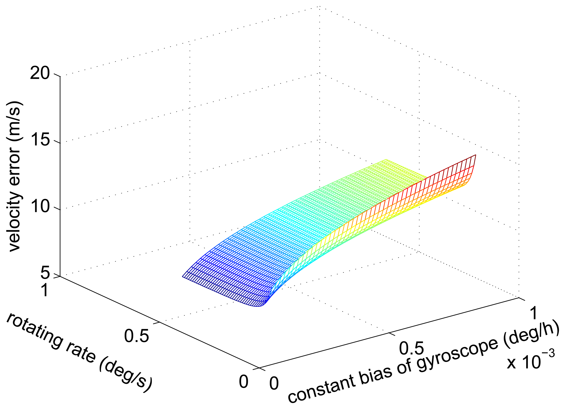
It is known that the amplitude of the velocity error caused by the gyroscope constant bias decreases with the increase of the rotating angular rate from Equations (16) and (19). Figure 3 shows the simulation results.

3.1.2. Velocity Error Caused by the Constant Bias of Accelerometers

The east velocity error caused by the accelerometer constant bias can be expressed in the frequency domain as:

$$\delta V_E^2(s)=M_1\cdot W_2(s)=\frac{s(s{\nabla }_{x0}-{\omega }_r{\nabla }_{y0})}{(s^2+{\omega }_s^2)(s^2+{\omega }_r^2)}$$

(20)

After the inverse Laplace transform and simplification, we get the east velocity error caused by the accelerometer constant bias in the time domain and shown as:

$$\delta V_E^2(t)=k_{31}cos{\omega }_{s}t+k_{32}sin{\omega }_{s}t+k_{33}cos{\omega }_{r}t+k_{34}sin{\omega }_{r}t$$

(21)

The amplitude of the east velocity error is expressed as:

$$A_{E2}({\omega }_r)=\sqrt{k_{31}^2+k_{32}^2+k_{33}^2+k_{34}^2}$$

(22)

where:

$$\begin{array}{cccc}{k}_{31}=-\frac{1}{{\omega }_r}{\nabla }_{y0};& k_{32}=-\frac{{\omega }_s}{{\omega }_r^2}{\nabla }_{x0};& k_{33}=\frac{1}{{\omega }_r}{\nabla }_{x0};& k_{34}=\frac{1}{{\omega }_r}{\nabla }_{y0}\end{array}$$

The north velocity error caused by the accelerometer constant bias can be expressed in the frequency domain as:

$$\delta V_N^2(s)=\frac{s({\omega }_r{\nabla }_{x0}+s{\nabla }_{y0})}{(s^2+{\omega }_s^2)(s^2+{\omega }_r^2)}$$

(23)

After the inverse Laplace transform and simplifying Equation (23), we get the east velocity error caused by the accelerometer constant bias in the time domain as:

$$\delta V_N^2(t)=k_{41}sin{\omega }_{r}t+k_{42}sin{\omega }_{s}t-k_{43}cos{\omega }_{r}t-k_{44}sin{\omega }_{s}t$$

(24)

The amplitude of the east velocity error is expressed as:

$$A_{N2}({\omega }_r)=\sqrt{k_{41}^2+k_{42}^2+k_{43}^2+k_{44}^2}$$

(25)

where:

$$\begin{array}{cccc}{k}_{41}=\frac{{\nabla }_{y0}}{{\omega }_r};& k_{42}=\frac{{\nabla }_{x0}}{{\omega }_r};& k_{43}=-\frac{{\nabla }_{x0}}{{\omega }_r};& k_{44}=-\frac{{\omega }_s{\nabla }_{y0}}{{\omega }_r^2}\end{array}$$

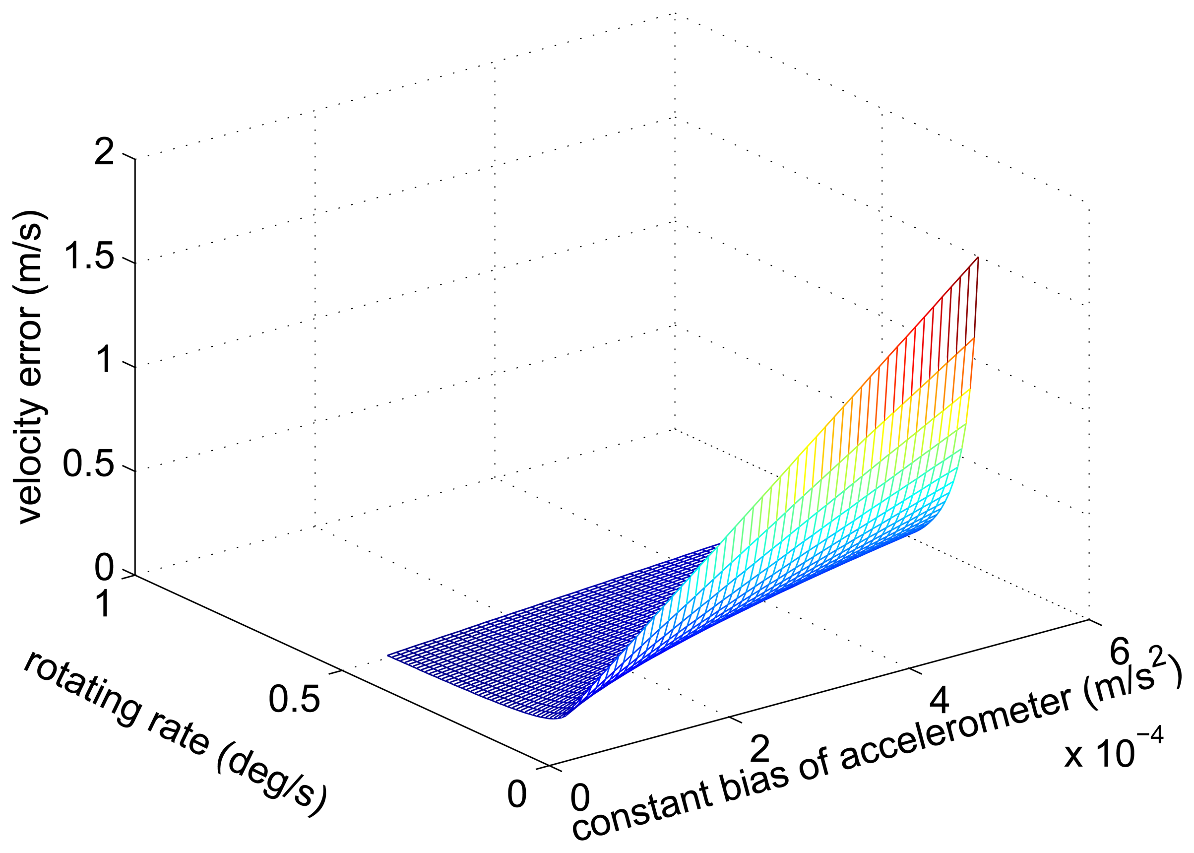
The conclusion is obtained from Equations (22) and (25) that the amplitude of the velocity error caused by the accelerometer constant bias decreases with the increase of the rotating angular rate. Figure 4 shows the simulation results.

3.1.3. Velocity Error Caused by the Scale Factor Error

The east velocity error caused by the scale factor error can be expressed in the frequency domain as:

$$\begin{array}{cc}\delta V_E^3(s)& =M_1\cdot W_3(s)\hfill \\ & \begin{array}{c}=\frac{g{\omega }_r{\omega }_{ie}cosL(s^2{\omega }_{ie}sinL-s^2{\omega }_r-{\omega }_r{\omega }_{ie}^2{cos}^{2}L)}{(s^2+{\omega }_s^2)(s^2+{\omega }_{ie}^2){(s^2+{\omega }_r^2)}^2}{K}_{gx}\hfill \\ -\frac{s^{2}g{\omega }_{ie}cosL(s^2+{\omega }_r{\omega }_{ie}sinL+{\omega }_{ie}^2{cos}^{2}L)}{(s^2+{\omega }_s^2)(s^2+{\omega }_{ie}^2){(s^2+{\omega }_r^2)}^2}{K}_{gy}+\frac{g{\omega }_{ie}^{2}sinLcosL({\omega }_{ie}sinL+{\omega }_r)}{s^2(s^2+{\omega }_s^2)(s^2+{\omega }_{ie}^2)}{K}_{gz}\end{array}\end{array}$$

(26)

After the inverse Laplace transform and simplifying Equation (26), we get the east velocity error caused by the scale factor error in the time domain as:

$$\delta V_E^3(t)=k_{51}sin{\omega }_{r}t+k_{52}sin{\omega }_{s}t+k_{53}sin{\omega }_{ie}t+k_{54}t$$

(27)

The amplitude of the east velocity error is expressed as:

$$A_{E3}({\omega }_r)=\sqrt{k_{51}^2+k_{52}^2+k_{53}^2+k_{54}^2}$$

(28)

where:

$$\begin{array}{l}\begin{array}{ccc}{k}_{51}=\frac{g{\omega }_{ie}^{2}sinLcosL}{{\omega }_r{\omega }_s^5}{K}_{gz};& k_{52}=\frac{g{\omega }_{ie}cosL}{{\omega }_r^3}{K}_{gx};& k_{53}=\frac{g{\omega }_{r}sinLcosL}{{\omega }_r^2}{K}_{gz};\end{array}\hfill \\ k_{54}=\frac{g{\omega }_{r}sinLcosL}{{\omega }_r^2}{K}_{gz}\hfill \end{array}$$

The north velocity error caused by the scale factor error can be expressed in the frequency domain as:

$$\begin{array}{cc}\delta V_N^3(s)& =M_2\cdot W_3(s)\hfill \\ & \begin{array}{l}=\frac{g{\omega }_{ie}cosL{\omega }_{r}s(s^2+{\omega }_r{\omega }_{ie}sinL)}{(s^2+{\omega }_s^2)(s^2+{\omega }_{ie}^2){(s^2+{\omega }_r^2)}^2}{K}_{gx}-\frac{s^{3}g{\omega }_{ie}cosL({\omega }_r+{\omega }_{ie}sinL)}{(s^2+{\omega }_s^2)(s^2+{\omega }_{ie}^2){(s^2+{\omega }_r^2)}^2}{K}_{gy}\hfill \\ -\frac{g{\omega }_{ie}cosL({\omega }_{ie}sinL+{\omega }_r)}{s(s^2+{\omega }_s^2)(s^2+{\omega }_{ie}^2)}{K}_{gz}\hfill \end{array}\end{array}$$

(29)

After the inverse Laplace transform and the simplification, we get the east velocity error caused by the scale factor error in the time domain as:

$$\delta V_N^3(t)=k_{61}cos{\omega }_{s}t+k_{62}cos{\omega }_{r}t+k_{63}$$

(30)

The amplitude of the east velocity error is expressed as:

$$A_{N3}({\omega }_r)=\sqrt{k_{61}^2+k_{62}^2+k_{63}^2}$$

(31)

where:

$$\begin{array}{ccc}{k}_{61}=-\frac{g{\omega }_{ie}^2{\omega }_{r}cosL}{{\omega }_s^4}{K}_{gz};& k_{62}=\frac{g{\omega }_{r}cosL}{{\omega }_s^2}{K}_{gz};& k_{63}=\frac{g{\omega }_{r}cosL}{{\omega }_s^2}{K}_{gz}\end{array}$$

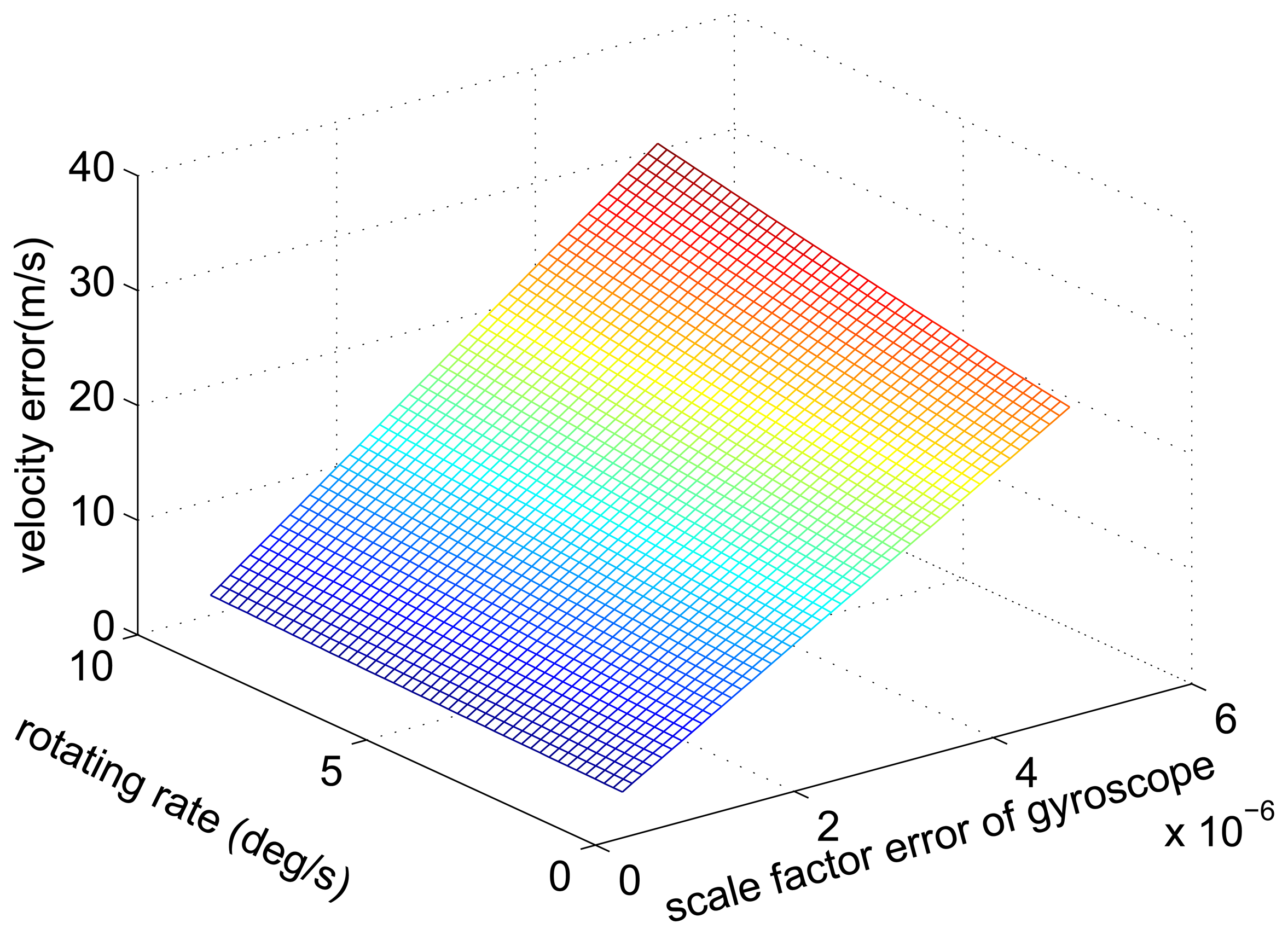
From Equations (28) and (31), we can draw a conclusion that the amplitude of the velocity error caused by the accelerometer constant bias increases with the increase of the rotating angular rate. Additionally, we plot the relationship between the amplitude of the velocity error, the scale factor error and the rotating angular rate as Figure 5.

3.1.4. Velocity Error Caused by the Installation Error

The east velocity error caused by the installation error can be expressed in the frequency domain as:

$$\begin{array}{ll}\delta V_E^4(s)\hfill & =M_1\cdot W_4(s)\hfill \\ \hfill & \begin{array}{l}=\frac{[g{\omega }_{ie}sinL{s}^2-g(s^2+{\omega }_{ie}^2{cos}^{2}L){\omega }_r]({\omega }_{ie}sinL+{\omega }_r)}{s(s^2+{\omega }_s^2)(s^2+{\omega }_{ie}^2)(s^2+{\omega }_r^2)}{\delta }_{xy}\hfill \\ -\frac{{\omega }_{ie}cosLs[g{\omega }_{ie}sinL{s}^2-g(s^2+{\omega }_{ie}^2{cos}^{2}L){\omega }_r]}{(s^2+{\omega }_s^2)(s^2+{\omega }_{ie}^2){(s^2+{\omega }_r^2)}^2}{\delta }_{xz}\hfill \\ -\frac{{\omega }_{ie}cosL{\omega }_r[g{\omega }_{ie}sinLs{\omega }_r+g(s^2+{\omega }_{ie}^2{cos}^{2}L)s]}{(s^2+{\omega }_s^2)(s^2+{\omega }_{ie}^2){(s^2+{\omega }_r^2)}^2}{\delta }_{yz}\hfill \\ +\frac{({\omega }_{ie}sinL+{\omega }_r)[g{\omega }_{ie}sinLs{\omega }_r+g(s^2+{\omega }_{ie}^2{cos}^{2}L)s]}{s(s^2+{\omega }_s^2)(s^2+{\omega }_{ie}^2)(s^2+{\omega }_r^2)}{\delta }_{yx}\hfill \\ +\frac{g{\omega }_{ie}^{2}sinL{cos}^{2}L}{(s^2+{\omega }_s^2)(s^2+{\omega }_{ie}^2)(s^2+{\omega }_r^2)}{\delta }_{zx}-\frac{g{\omega }_{ie}^{3}sinL{cos}^{2}L{\omega }_r}{s(s^2+{\omega }_s^2)(s^2+{\omega }_{ie}^2)(s^2+{\omega }_r^2)}{\delta }_{zy}\hfill \end{array}\hfill \end{array}$$

(32)

After the inverse Laplace transform and simplification, we get the east velocity error caused by the installation error in the time domain as:

$$\delta V_E^4(t)=k_{71}sin{\omega }_{r}t+k_{72}cos{\omega }_{r}t+k_{73}cos{\omega }_{s}t+k_{74}sin{\omega }_{ie}t+k_{75}cos{\omega }_{ie}t+k_{76}$$

(33)

The amplitude of the east velocity error is expressed as:

$$A_{E4}({\omega }_r)=\sqrt{k_{71}^2+k_{72}^2+k_{73}^2+k_{74}^2+k_{75}^2+k_{76}^2}$$

(34)

where:

$$\begin{array}{c}\begin{array}{ccc}{k}_{71}=-\frac{g{\delta }_{yx}}{{\omega }_r^2};& k_{72}=-\frac{g{\delta }_{xy}}{{\omega }_r^2};& k_{73}=-\frac{g{\omega }_{ie}sinL{cos}^{2}L{\delta }_{zy}}{{\omega }_s^4{\omega }_r};\end{array}\\ \begin{array}{ccc}{k}_{74}=\frac{gsinL{\delta }_{yx}}{{\omega }_s^2};& k_{75}=-\frac{gsinL{\delta }_{xy}}{{\omega }_s^2};& k_{76}=-\frac{gsinL{\delta }_{yx}}{{\omega }_s^2{\omega }_r^5}\end{array}\end{array}$$

The north velocity error caused by the installation error can be expressed in the frequency domain as:

$$\begin{array}{ll}\delta V_N^4(s)\hfill & =M_2\cdot W_4(s)\hfill \\ \hfill & \begin{array}{c}=\frac{g(s^2-{\omega }_r{\omega }_{ie}sinL)({\omega }_{ie}sinL+{\omega }_r)}{(s^2+{\omega }_s^2)(s^2+{\omega }_{ie}^2)(s^2+{\omega }_r^2)}{\delta }_{xy}-\frac{s^{2}g{\omega }_{ie}cosL(s^2-{\omega }_r{\omega }_{ie}sinL)}{(s^2+{\omega }_s^2)(s^2+{\omega }_{ie}^2){(s^2+{\omega }_r^2)}^2}{\delta }_{xz}\\ -\frac{({\omega }_r+{\omega }_{ie}sinL)s^{2}g{\omega }_{ie}cosL{\omega }_r}{(s^2+{\omega }_s^2)(s^2+{\omega }_{ie}^2){(s^2+{\omega }_r^2)}^2}{\delta }_{yz}+\frac{gs{({\omega }_r+{\omega }_{ie}sinL)}^2}{(s^2+{\omega }_s^2)(s^2+{\omega }_{ie}^2)(s^2+{\omega }_r^2)}{\delta }_{yx}\\ -\frac{sg\omega i{e}^2{cos}^{2}L}{(s^2+{\omega }_s^2)(s^2+{\omega }_{ie}^2)(s^2+{\omega }_r^2)}{\delta }_{zx}+\frac{g{\omega }_r{\omega }_{ie}^2{cos}^{2}L}{(s^2+{\omega }_s^2)(s^2+{\omega }_{ie}^2)(s^2+{\omega }_r^2)}{\delta }_{zy}\end{array}\hfill \end{array}$$

(35)

After the inverse Laplace transform and simplification, we get the north velocity error caused by the installation error in the time domain as:

$$\delta V_N^4(t)=k_{81}cos{\omega }_{r}t+k_{82}cos{\omega }_{s}t+k_{83}cos{\omega }_{i}et+k_{84}sin{\omega }_{r}t\cdot t$$

(36)

The amplitude of the north velocity error is expressed as:

$$A_{N4}({\omega }_r)=\sqrt{k_{81}^2+k_{82}^2+k_{83}^2+k_{84}^2}$$

(37)

where:

$$\begin{array}{cccc}{k}_{81}=\frac{2g{\delta }_{yx}}{{\omega }_r^4};& k_{82}=-\frac{g{\delta }_{yx}}{{\omega }_r^2{\omega }_s^2};& k_{83}=-\frac{g{\delta }_{yx}}{{\omega }_r^2{\omega }_s^2};& k_{84}=-\frac{g{\delta }_{yx}}{2{\omega }_r^2}\end{array}$$

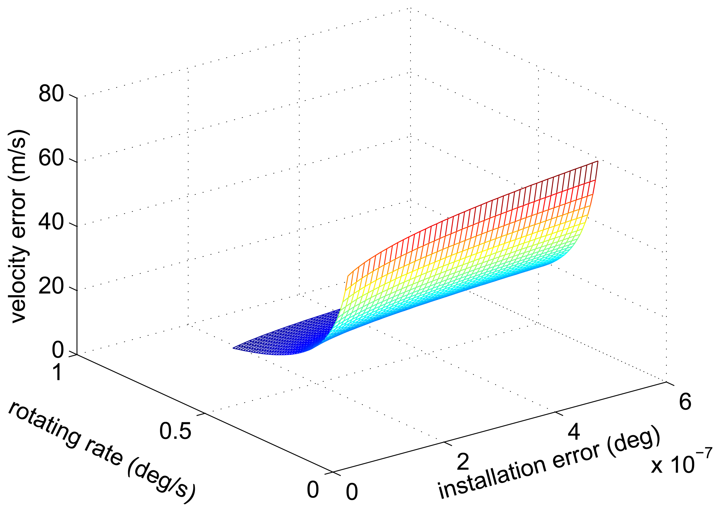
From Equations (34) and (37), we can draw a conclusion that the amplitude of the velocity error caused by the installation error increase with the increase of rotating angular rate. Additionally, we plot the relationship between the amplitude of the velocity error, the installation error and the rotating angular rate as Figure 6.

3.2. Optimal Design Method for the Angular Rate

Section 3.1 is focused on the relationship between the velocity error, three different kinds of inertial sensors errors and the rotating angular rate. In this part, we will propose the optimal design method of the rotating angular rate.

When the RSINS rotates at a constant speed, the amplitude of the velocity error can be expressed as:

$$A({\omega }_r)=\sqrt{A_1^2({\omega }_r)+A_2^2({\omega }_r)+A_3^2({\omega }_r)+A_4^2({\omega }_r)}$$

(38)

where $\begin{array}{cc}{A}_j({\omega }_r)=\sqrt{A_{Ej}^2({\omega }_r)+A_{Nj}^2({\omega }_r)}& (j=1,\cdots ,4)\end{array}$.

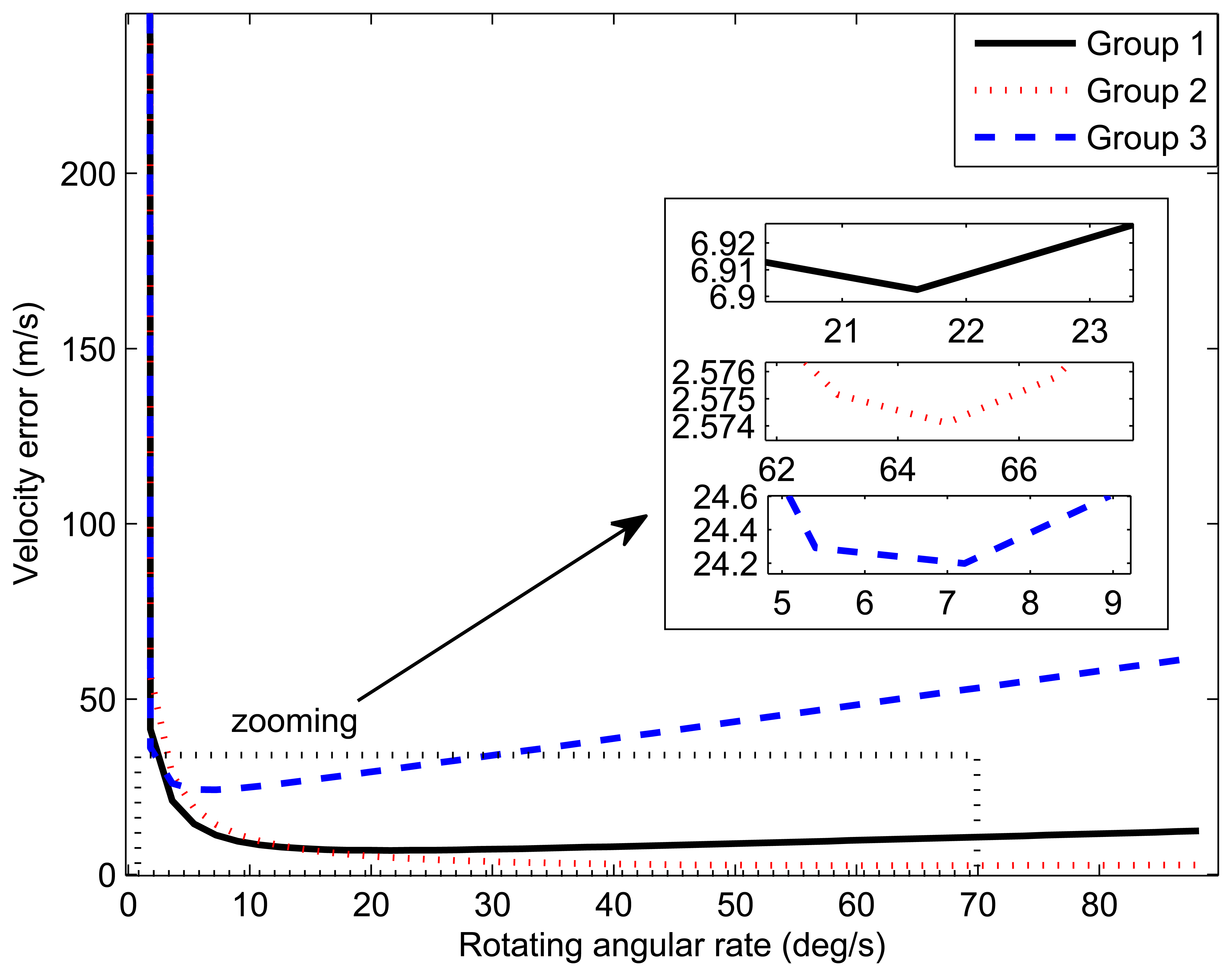
From the Equation (38), it is known that the amplitude of the velocity error can be expressed as a function of the inertial sensor error and the rotating angular rate. Therefore, for the purpose of ensuring the minimum of the velocity error amplitude, the rotating angular rate should match the error of the inertial sensors. In order to verify and determine this matching relationship, we will design three groups of inertial sensor performances and calculate the optimal rotating angular rate of each group with MATLAB. Taking “MARINS”, a high-precision INS manufactured by IXBlue, as an example, its positioning accuracy is 1 nm/24 h. It can be inferred that the constant bias and the scale factor error of its gyroscopes are lower than 0.01 °/h and 1 × 10^-6 (°/h)^-1, respectively. On the other hand, considering the real INS, the constant bias accelerometer is lower than 9.8 × 10^-4 m/s², and the installation error of gyroscopes is lower than 1 × 10^-9 °/h. Therefore, on the basis of the above, the simulation parameters are set as Tables

Table 1. Inertial sensor performance (Group 1).

Sensor Error	Parameter Value
Constant bias of gyroscope	0.01 (°/h)
Constant bias of accelerometer	9.8 × 10-4 (m/s2)
Scale factor error of gyroscope	1 × 10-6 (°/h)-1
Installation error of gyroscope	1 × 10-9 (°/h)

-

Table 3. Inertial sensor performance (Group 3).

Sensor Error	Parameter Value
Constant bias of gyroscope	0.002 (°/h)
Constant bias of accelerometer	1.96 × 10-4 (m/s2)
Scale factor error of gyroscope	5 × 10-6 (°/h)-1
Installation error of gyroscope	2 × 10-10 (°/h)

, respectively.

Figure 7 depicts the relationship between the amplitude of the velocity error and the rotating angular rate by MATLAB. The value of the horizontal axis corresponding to the minimum of the curve is the optimal rotating angular rate. The optimal rotating angular rates of these three groups are summarized in

Table 4. Optimal rotating rates with different simulation conditions.

Group	Optimal rotating angular rate
1	21.6°/s
2	64.8°/s
3	7.2°/s

.

4. Numerical Simulations

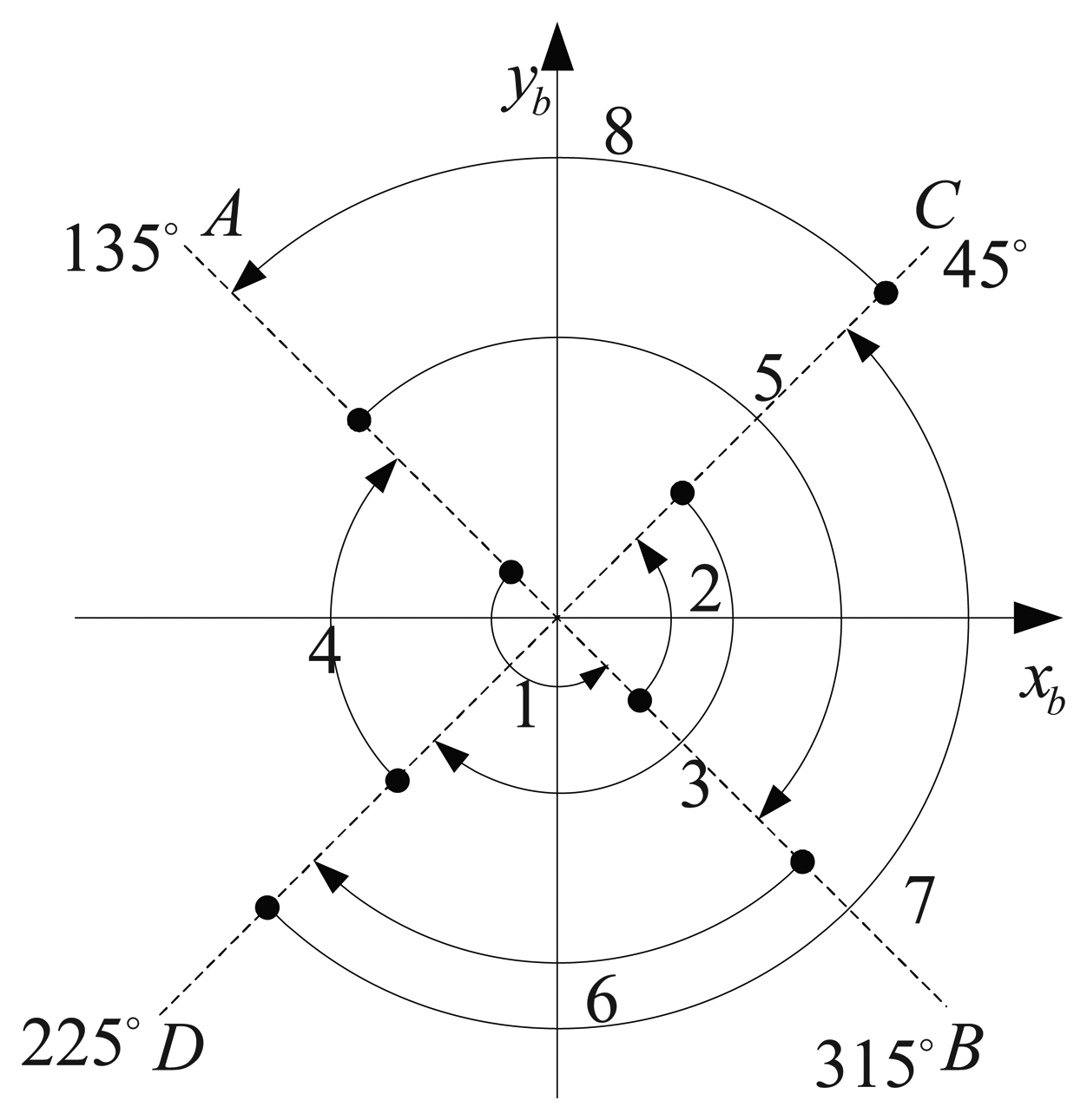
The optimal design method of the rotating angular rate is proposed in Section 3. The theoretical optimal rotating angular rates corresponding to three different groups of inertial sensor errors are obtained in terms of this method. In order to verify the correctness of the former conclusions, simulations are carried out in this section. The rotating scheme is proposed as shown in Figure 8. The turntable rotates the IMU back and forth along the azimuth axis through four orthogonal positions. The dwell time in each position is 45 s [25].

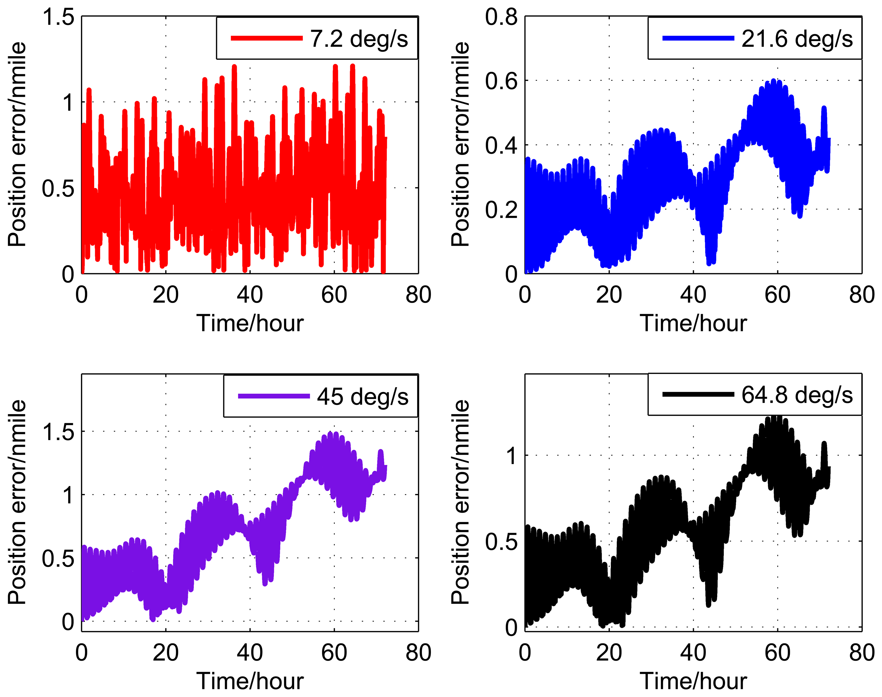
The performances of inertial sensors are described in Tables 1,

Table 2. Inertial sensor performance (Group 2).

Sensor Error	Parameter Value
Constant bias of gyroscope	0.05 (°/h)
Constant bias of accelerometer	4.9 × 10-3 (m/s2)
Scale factor error of gyroscope	0.2 × 10-6 (°/h)-1
Installation error of gyroscope	5 × 10-9 (°/h)

, and 3. The rotating angular rates are designed as 7.2 °/s, 21.6 °/s, 45 °/s and 64.8 °/s; as 21.6 °/s, 64.8 °/s and 7.2 °/s are the optimal rotating rate of Groups 1-3, respectively, and 45 °/s is chosen for comparison.

Figures 9, 10, and 11 show the simulation results of the position error of different groups. The simulation duration is 72 h.

Table 5. Position error (Group 1).

Rotating angular rate (°/s)	7.2	21.6	45	64.8
Position error (nmile/72h)	1.2	0.6	1.5	1.3

,

Table 6. Position error (Group 2).

Rotating angular rate (°/s)	7.2	21.6	45	64.8
Position error (nmile/72h)	5.0	0.9	1.0	0.6

, and

Table 7. Position error (Group 3).

Rotating angular rate (°/s)	7.2	21.6	45	64.8
Position error (nmile/72h)	2.5	3.0	5.0	4.2

summarize the simulation results.

It can be seen from Figure 9 and Table 5 that the position error of Group 1 with a rotating angular rate of 21.6 °/s is lower than the other rotating angular rates. From Figure 10 and Table 6, it can be seen that the position error of Group 2 with a rotating angular rate of 64.8 °/s is lower than the other rotating angular rates. From Figure 10 and Table 6, we can see that the position error of Group 3 with a rotating angular rate of 7.2 °/s is lower than the other rotating angular rates. The simulation results are in accordance with the conclusions of Section 3.

5. Experimental Study

In order to verify the effectiveness of the method, experiments were done in Songhuajiang River in Harbin, as shown in Figure 12. Experimental equipment, as shown in Figure 13, included SINS, single-axis turn-table, GPS, computers and a UPS. The SINS is manufactured by Harbin Engineering University, and the main parameters are shown in

Table 8. The main parameters of the fiber optics gyroscope.

Performance	Parameters
Dynamic range	±100°/s
Bias stability	≤ 0.003 °/h
Random walk	$\le 0.001°/\sqrt{h}$
Scale factor error	≤ 5 ppm

and

Table 9. The main parameters of the accelerometer.

Performance	Parameters
Dynamic range	±4g
Bias stability	≤ 1 × 10-5

. The single-axis turn-table is manufactured by Beijing Precision Engineering Institute for Aircraft Industry, and the main parameters are shown in

Table 10. Performances of the 920E single axis velocity and position turntable.

Performance	Parameters
Diameter	450 m
Carrying capacity	weight 50 kg
Rotating accuracy	±2″
Rotating range	continues and infinite
Location accuracy	±3″
Location definition	0.0001°
Speed range	0.005 - 200 °/s
Speed accuracy	5 × 10-5 (360°average)
Speed accuracy	5 × 10-4 (10°average)
Speed accuracy	1 × 10-2 (l°average)

.

5.1. Experimental Scheme

With the optimal design method proposed in this paper, the optimal angular rate for the experimental system is calculated to be 7 °/s. Therefore, three angular rates, 2 °/s, 7 °/s and 20 °/s, are used in the experiments for comparison. The experimental duration is 72 h, and the rotating scheme is the same as that in Section 4.1.

The rotating angular rate is not constant in a real system, since the IMU needs to reverse the rotating direction. The positioning accuracy of RSINS is influenced by the IMU turned angle in the variable angular rate process [26]. Additionally, the analysis results show that the error will be minimum in the process of the varied angle rate when the IMU's turned angle achieves 0.2π. In order to eliminate the effects of the variable angular rate, the angular accelerations are set as 0.1 °/s², 0.7 °/s² and 5.6 °/s², respectively, in the experiment.

5.2. Experimental Results and Analysis

Figures 14-16 show the position error of three experiments.

From the theoretical analysis of Section 3, it is known that the rotation modulation method can only reduce the amplitude of the oscillation error and the slope of the ramp error, but not eliminate them. Therefore, it can be seen from Figures 14-16 that the resulting position error comprises a ramp error with superimposed Schuler oscillation and Earth rotation oscillation, and the oscillation periods are 84.4 min and 24 h. From

Table 11. Experimental results.

Rotating angular rate (°/s)	2	7	20
Position error (nmile/72h)	14.7	6.4	19.6

, it can be seen obviously that the position error of Experiment II is much less than the other two. The experimental results are consistent with the theoretical analysis of Section 3.

6. Conclusions and Future Work

This paper presented a rotating angular rate optimal design method of the RSINS. Firstly, the RSINS and the principle of the rotation modulation were introduced, and the inertial sensor errors were modeled. Secondly, the relation between the velocity error and the angular rate was worked out using the Laplace transform and the inverse Laplace transform. The optimal rotating angular rate method was also proposed based on the relationship above. Thirdly, simulations were conducted, and the results confirmed that the optimal rotating angular rate could be computed correctly with this method. Navigation experiments were done, and the results of the positioning error confirmed the effectiveness and correctness of the theoretical analyze. However, the experimental time was just 72 h, because of the limitations of experimental conditions. As a result, we plan to do more further experiments, which will last a longer time, if the experimental conditions permit, in the future. On the other hand, the results of the simulations were superior to that of the experiments. The reason may be that an error of the initial alignment, which is ignored, in the simulations may occur. The initial alignment error is not the main factor of the rotating angular rate optimal design method from the analysis of simulations and experimental results. Even so, we will model the initial alignment error and focus on its impact on the RSINS in the future.

References

- Ishibashi, S.; Tsukioka, S.; Yoshida, H.; Hyakudome, T.; Sawa, T.; Tahara, J.; Aoki, T.; Ishikawa, A. Accuracy Improvement of an Inertial Navigation System Brought about by the Rotational Motion. Proceedings of OCEANS 2007-Europe, Aberdeen, UK, 18–21 June 2007; pp. 1–5.
- Levinson, E.; Ter Horst, J.; Willcocks, M. The Next Generation Marine Inertial Navigator is Here Now. Proceedings of the IEEE Position Location and Navigation Symposium, Las Vegas, NV, USA, 11–15 April 1994; pp. 121–127.
- Tucker, T.; Levinson, E. The AN/WSN-7B Marine Gyrocompass/Navigator. Proceedings of the 2000 National Technical Meeting of the Institute of Navigation, Anaheim, CA, USA, 26–28 January 2000; pp. 348–357.
- Titterton, D.; Weston, J. Strapdown Inertial Navigation Technology, 2nd ed; The Institution of Electronical Engineers: Reston, VA, USA, 2004. [Google Scholar]
- Gao, W.; Zhang, Y.; Wang, J. A Strapdown Interial Navigation System/Beidou/Doppler Velocity Log Integrated Navigation Algorithm Based on a Cubature Kalman Filter. Sensors 2014, 14, 1511–1527. [Google Scholar]
- Lahham, J.; Brazell, J. Acoustic Noise Reduction in the MK 49 Ship's Inertial Navigation System (SINS). Proceedings of the Position Location and Navigation Symposium, 1992. Record. 500 Years After Columbus-Navigation Challenges of Tomorrow. IEEE PLANS'92., IEEE, Monterey, CA, USA, 23–27 March 1992; pp. 32–39.
- Levinson, E.; Majure, R. Accuracy Enhancement Techniques Applied to the Marine Ring Laser Inertial Navigator (MARLIN). Navigation 1987, 34, 64–86. [Google Scholar]
- Gao, Z.Y. Initial Navigation System Technology; Tsinghua University Press: Beijing, China, 2012; p. p. 290. [Google Scholar]
- Heckman, D.W.; Baretela, L. Improved Affordability of High Precision Submarine Inertial Navigation by Insertion of Rapidly Developing Fiber Optic Gyro Technology. Proceedings of the Position Location and Navigation Symposium, IEEE 2000, San Diego, CA, USA, 13–16 March 2000; pp. 404–410.
- Ben, Y.Y.; Chai, Y.L.; Gao, W.; Sun, F. Analysis of Error for a Rotating Strap-Down Inertial Navigation System with Fibro Gyro. J. Mar. Sci. Appl. 2010, 9, 419–424. [Google Scholar]
- Che, L.; Sun, W.; Xu, A. Influence of IMU Rotation Angular Rate on Navigation Accuracy of Rotary SINS. Chin. J. Sci. Instrum. 2012, 33, 1041–1047. [Google Scholar]
- Sun, F.; Wang, Q.; Qi, Z. Effect of Angle Variable Motion on Rotation Strapdown Inertial Navigation Systems. J. Huazhong. Univers. Sci. Technol. 2013, 41, 31–35. [Google Scholar]
- Adams, G.; Gokhale, M. Fiber Optic Gyro Based Precision Navigation for Submarines. Proceedings of the AIAA Guidence, Navigation and Control Conference, Denver, CO, USA, 14–17 August 2000.
- Ben, Y.; Sun, F.; Gao, W.; Yu, F. Generalized Method for Improved Coning Algorithms using Angular Rate. Aerosp. Electron. Syst., IEEE Trans. 2009, 45, 1565–1572. [Google Scholar]
- Zha, F.; Xu, J.N.; Hu, B.Q.; Qin, F.J. Error Analysis for SINS with Different IMU Rotation Scheme. Proceedings of the Informatics in Control, Automation and Robotics (CAR), 2010 2nd International Asia Conference on, Wuhan, China, 6–7 March 2010; pp. 422–425.
- Zha, F.; Hu, B.R.; Qin, F.J.; Luo, Y.B. A Rotating Inertial Navigation System with the Rotating Axis Error Compensation Consisting of Fiber Optic Gyros. Optoelectron. Lett. 2012, 8, 146–149. [Google Scholar]
- Liu, F.; Wang, W.; Wang, L.; Feng, P. Error Analyses and Calibration Methods with Accelerometers for Optical Angle Encoders in Rotational Inertial Navigation Systems. Appl. Opt. 2013, 52, 7724–7731. [Google Scholar]
- Yu, H.; Wu, W.; Wu, M.; Feng, G.; Hao, M. Systematic Angle Random Walk Estimation of the Constant Rate Biased Ring Laser Gyro. Sensors 2013, 13, 2750–2762. [Google Scholar]
- Ishibashi, S. The Improvement of the Prescision of an Inertial Navigation System for AUV based on the Neural Network. Proceedings of the OCEANS 2006-Asia Pacific, Singapore, 16–19 May 2007; pp. 1–6.
- Sun, G.; Wang, M.; Huang, L.; Shen, L. Generating Multi-Scroll Chaotic Attractors via Switched Fractional Systems. Circuits. Syst. Signal. Process. 2011, 30, 1183–1195. [Google Scholar]
- Sun, F.; Lan, H.; Yu, C.; El-Sheimy, N.; Zhou, G.; Cao, T.; Liu, H. A Robust Self-Alignment Method for Ship's Strapdown INS under Mooring Conditions. Sensors 2013, 13, 8103–8139. [Google Scholar]
- Sun, G.; Ge, D.; Wang, S. Induced L2 Norm Control for LPV System with Specified Class of Disturbance Inputs. J. Frankl. Inst. 2013, 350, 331–346. [Google Scholar]
- Wang, B.; Xiao, X.; Xia, Y.; Fu, M. Unscented Particle Filtering for Estimation of Shipboard Deformation Based on Inertial Measurement Units. Sensors 2013, 13, 15656–15672. [Google Scholar]
- Sun, G.; Wang, M.; Wu, L. Unexpected Results of Extended Fractional Kalman Filter for Parameter Identification in Fractional Order Chaotic sSystems. Int. J. Innov. Comput. Inf. Control. 2011, 7, 5341–5352. [Google Scholar]
- Sun, W.; Gao, Y. Fiber-Based Rotary Strapdown Inertial Navigation System. Opt. Eng. 2013, 52, 076106–076106. [Google Scholar]
- Yu, F.; Sun, Q.; Zhang, Y.; Zu, Y. The Optimization Design of the Angular Rate and Acceleration Based on the Rotary SINS. Proceedings of the Control Conference (CCC), 2013 32nd Chinese, Xi'an, China, 26–28 July 2013; pp. 4969–4973.