3.1. Network Architecture
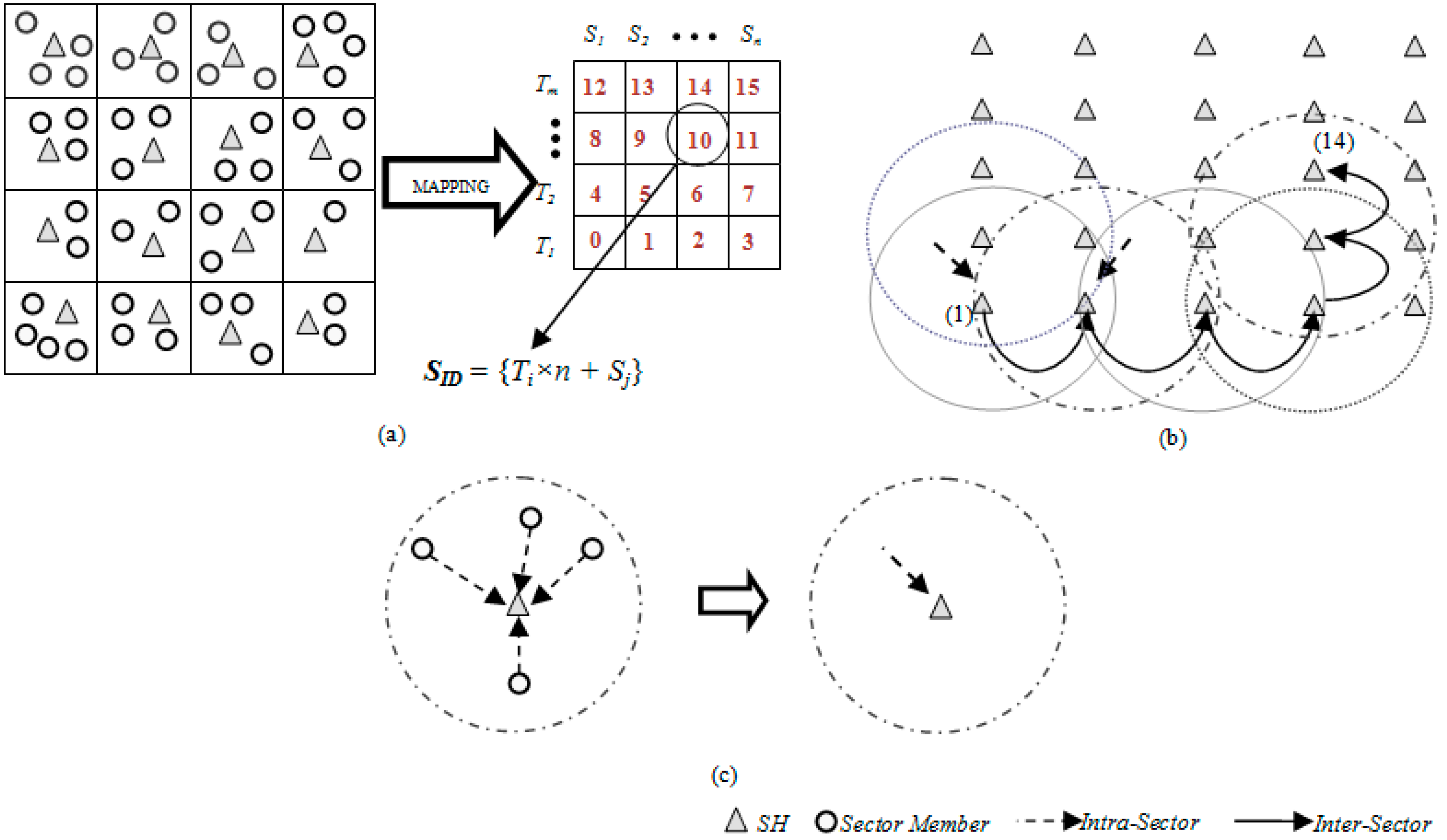
The surface/platter of a magnetic disk storage device consisting of tracks and sectors provides an interesting approach that may be applied to a large scale WSN. This assumption led to a Disk Based Data Centric Storage (DBDCS) architecture, as shown in
Figure 1a, dividing the rectangular field into a matrix of storage cells (referred to as a sector) where row and column represent track (
Ti) and sector (
Sj), respectively. In DBDCS, the covered network is considered as one of the storage surface and sector is considered as the core cell of storage. However, unlike magnetic storage disk, in DBDCS, the header file for data mapping is not located in one single particular location rather a dynamic mapping algorithm is used using hashing. Hence, each SH could calculate the target sector to read/write corresponding data. The physical deployment is mapped to an
m x n matrix, where
m is the number of tracks and
n is the number sectors for each track. Hence, the nodes in the network are divided into
S (mxn) sectors, each comprising a Sector Head (SH) and sector members that communicate
via one hop to the SH (see
Figure 1c), where
SHi ϵ [1…
S]. Each node is configured to be aware of the deployment layout by knowing: (1) All SHs are assigned with the sector number as a virtual address and node id, and (2) All member nodes know their own node id and number of tracks (
m) and sectors (
n) of the network field. As shown in
Figure 1b, the intra-sector communication (
i.e., communication from sector members to
SH or
vice-versa) is constrained to one hop while inter-sector transmission is multi-hop. For simplification, the sensor nodes inside each sector are not shown explicitly in
Figure 1b. Instead, an aggregated link (see
Figure 1c) is shown to represent the total traffic from member nodes to head node.
Figure 1.
(a) DBS mapping; (b) inter-sector communication; and (c) intra-sector member node to head node communication.
Figure 1.
(a) DBS mapping; (b) inter-sector communication; and (c) intra-sector member node to head node communication.
3.2. Metric-Based Searching
Metric space
M can be defined as a pair
M = (
D,
d), where
D is the domain of objects and
d is the
distance function—d: D ×
D →
R satisfying the following constraints for all objects
a,
b,
c ϵ
D:
In this metric space, two types of similarity queries can be defined including range query
Range(
q,
r) and
K-nearest neighbor search
KNN(
q,
k) by the resultant set
X, considering
to be a finite set of indexed objects:
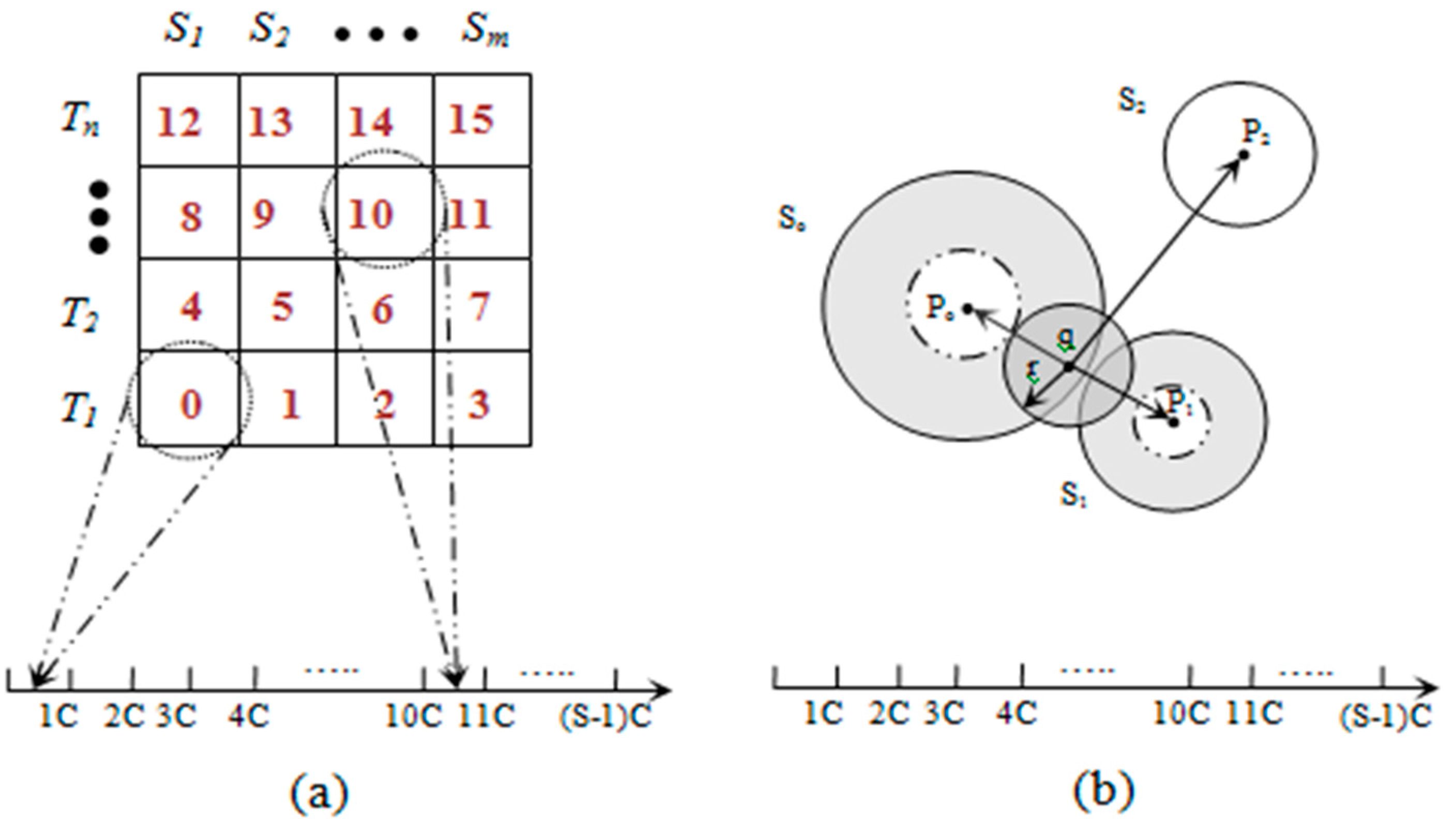
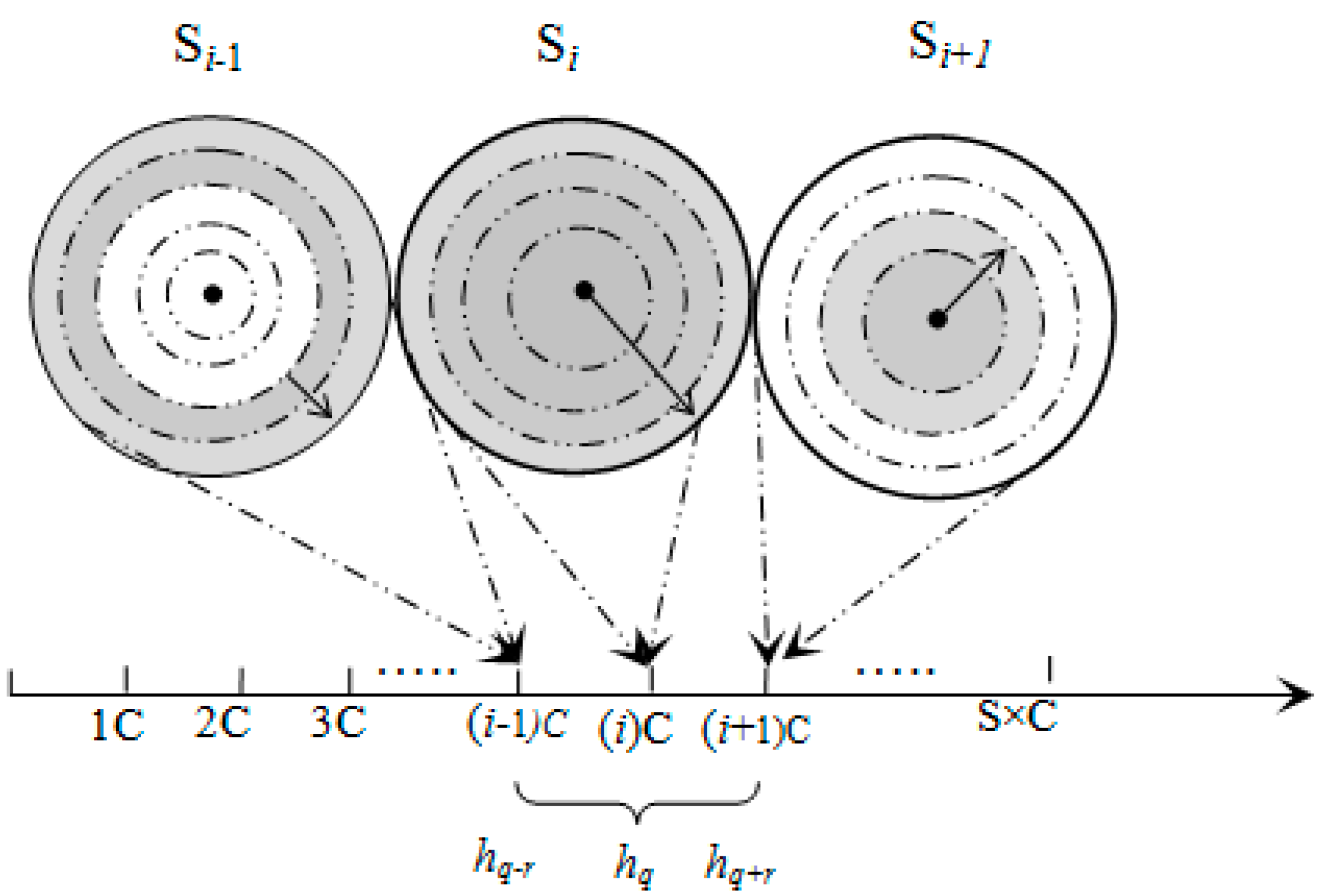
The data space can be divided into
S segments (
S is the total number of sectors) with a pivot point, denoted by
Pi, for each sector
Si. The
iDistance key for an object
x ϵ
D can be defined as (
Figure 2a):
In Equation (4),
c is the separating constant for individual sectors. Given
q ϵ
D, the range query for
q with the range of
r can be defined as (
Figure 2b):
In Equation (5),
q denotes the query point and
Pi denotes the pivot point for
SHi where
Pi ≤
q ≤
Pi+1. Therefore, after locating the target sector (
SHi), the conceptual range can be defined by Equation (5) and is illustrated in
Figure 2b. The axis showed in
Figure 2 represents the one dimensional data space that has been divided into
S segments, where each sector is mapped to a segment.
Figure 2.
(a) Data mapping; and (b) range query example.
Figure 2.
(a) Data mapping; and (b) range query example.
3.3. Data Processing and Mapping
A sensed event
E can be defined by an
l-dimensional tuple, (
A1,
A2,
A3,
…,
Al) where
denotes the
gth attribute and
DAg is the domain of attribute
Ag. Each member node of a sector transmits the sensed event as an
l-dimensional tuple
, where 1 ≤
i ≤
Mk,
Mk is the total number of member nodes in the
kth sector and
vij denotes the value of the
jth attribute received from
ith member node of the
kth sector. The corresponding SH, after collecting tuples from all the member nodes, aggregates them at the end of each epoch before finding the target SH mapping
. Hence, after aggregation at epoch
tHere, it is assumed that the attribute’s aggregated values of ψ
i have been normalized to be between the range of 0 and 1. From
Figure 1a, lets consider 6th (
k = 6) sector, where
M6 = 3. If the total number of attribute is 3 then for any particular round (for example
t = 2), Equation (6) can be illustrated as shown in
Table 2.
Table 2.
Illustration of Equations (6) and (7).
Table 2.
Illustration of Equations (6) and (7).
| Member Node | First Attribute | Second Attribute | Third Attribute |
|---|
| 1 | v11 | v12 | v13 |
| 2 | v21 | v22 | v23 |
| 3 | v31 | v32 | v33 |
| After applying Equations (6) and (7) |
| | max (v11, v21, v31) | max (v12, v22, v32) | max (v13, v23, v33) |
| min (v11, v21, v31) | min (v12, v22, v32) | min (v13, v23, v33) |
| avg (v11, v21, v31) | avg (v12, v22, v32) | avg (v13, v23, v33) |
As shown in
Table 3, weights have been assigned to different attributes based on their importance in the event description. Hence, an attribute with higher weight has greater influence on the similarity among events.
Table 3.
Weight settings.
Table 3.
Weight settings.
| Attribute | Weight |
|---|
| A1 | W1 |
| A2 | W2 |
| .... | .... |
| Al | wl |
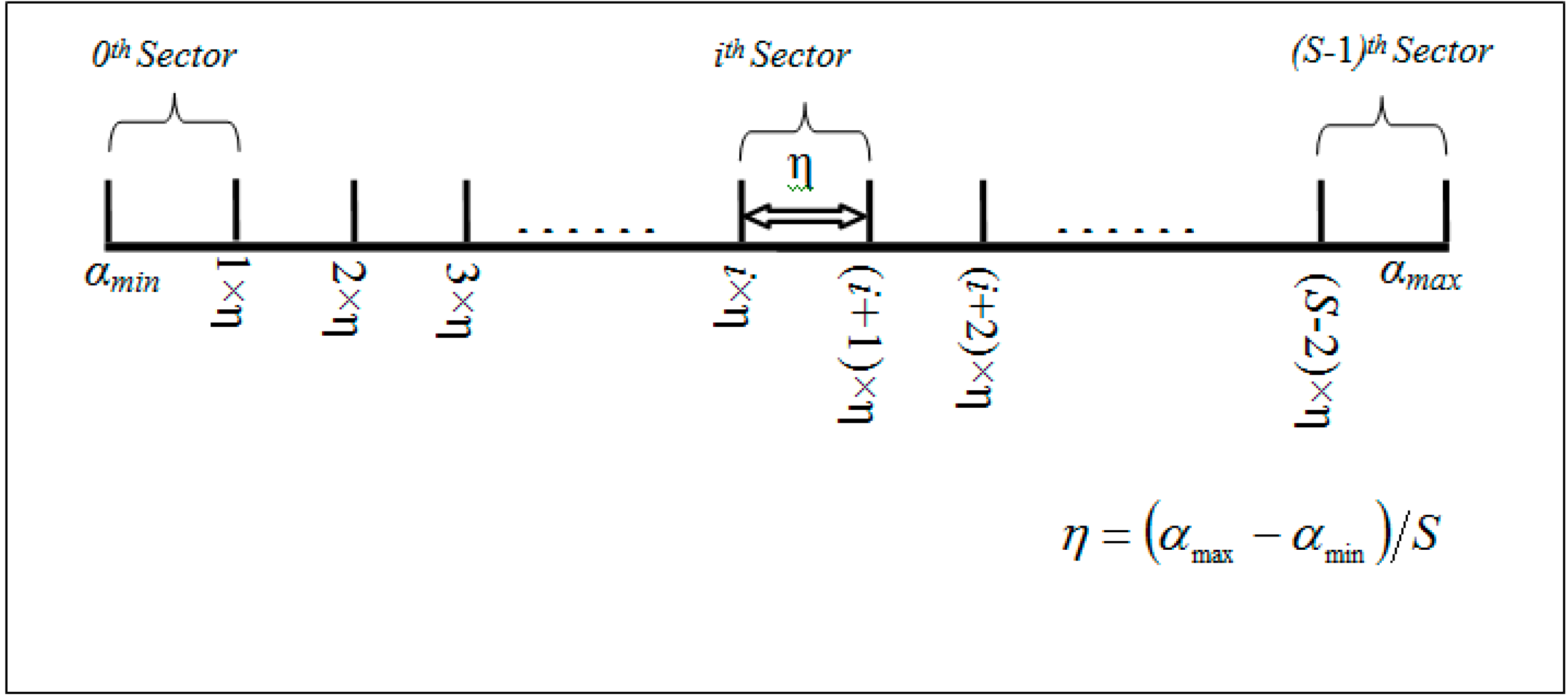
3.3.1. Pivot Point Generation
The domain of the one dimensional derived hash key
HD of an aggregated
l-dimensional sensed event can be defined by α (α
min, α
max) as illustrated in
Figure 3. In Equations (8)–(11), A
i(min), A
i(max), A
i(avg) and A
i(θ) denote the minimum, maximum, average and threshold value of
ith attribute. The center of mass (COM), denoted by β, is derived in Equation (10) to find the normalized center point of the domain of the hash key
HD whereas δ is the separating factor between two pivot point. However, in order to balance the load among sectors, it is important to find the range where the concentration of the data points is high. Hence, β and δ can be used to find this COM range, denoted by β (β
range-min, β
range-max) as shown in Equation (12):
Thus, the separating step, denoted by η, between two pivot points in the COM range can be defined by:
Thus the pivot points for
S sectors can be defined in each sector head by (Algorithm 1):
Figure 3.
Pivot point generation example.
Figure 3.
Pivot point generation example.
3.3.2. Mapping
Given
l attributes in an attribute list associated with weight
wj (1 ≤
j ≤
l) in a WSN application, the source
SHk generates the hash value by:
Hence, after each epoch, SHk forwards the aggregated event where t denotes the epoch number, to the destination sector head denoted by SHi where, Pi ≤ h ≤ Pi+1 and Pi and Pi+1 is the lower and upper limit of ith sub-interval, respectively.
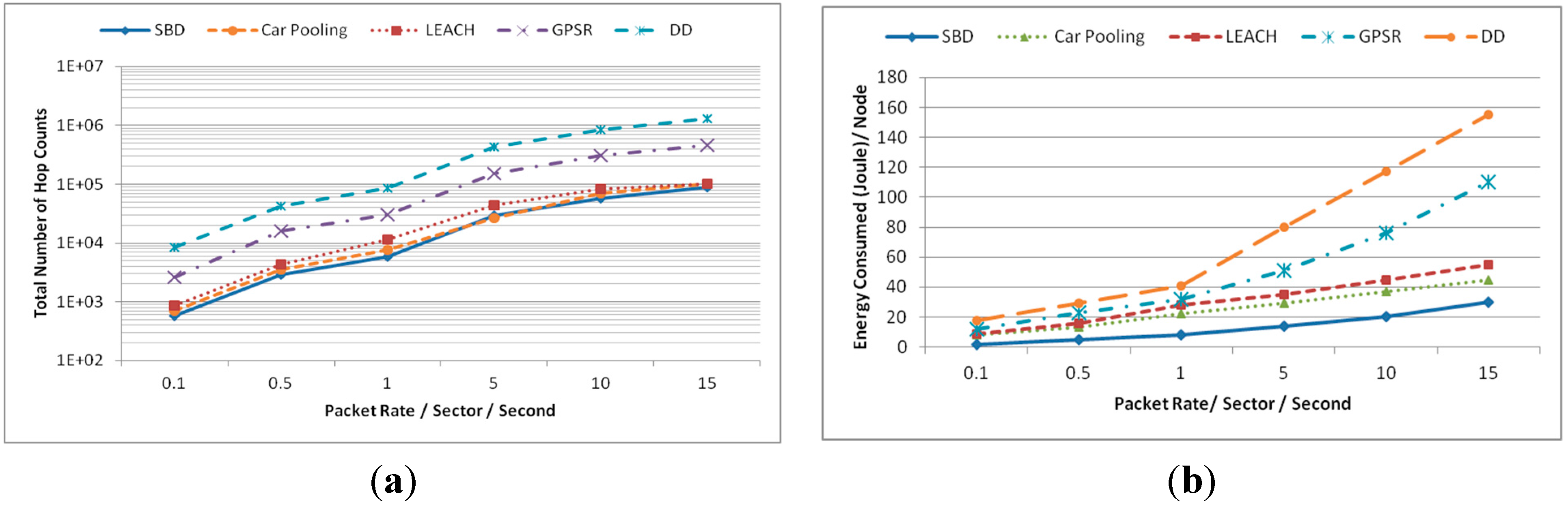
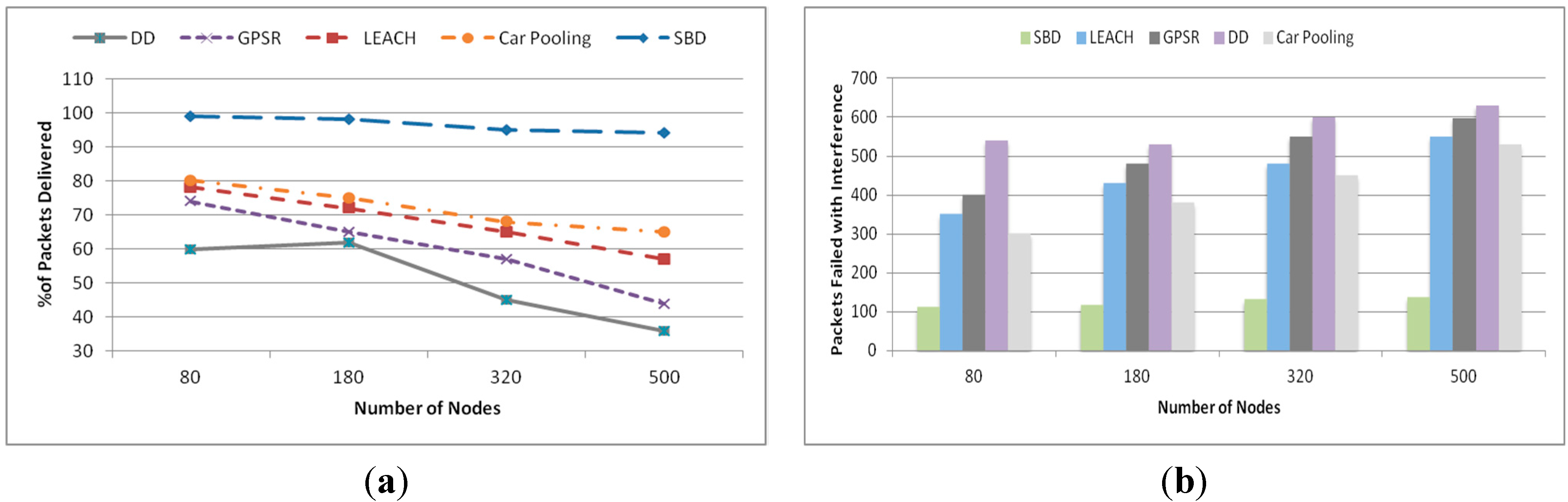
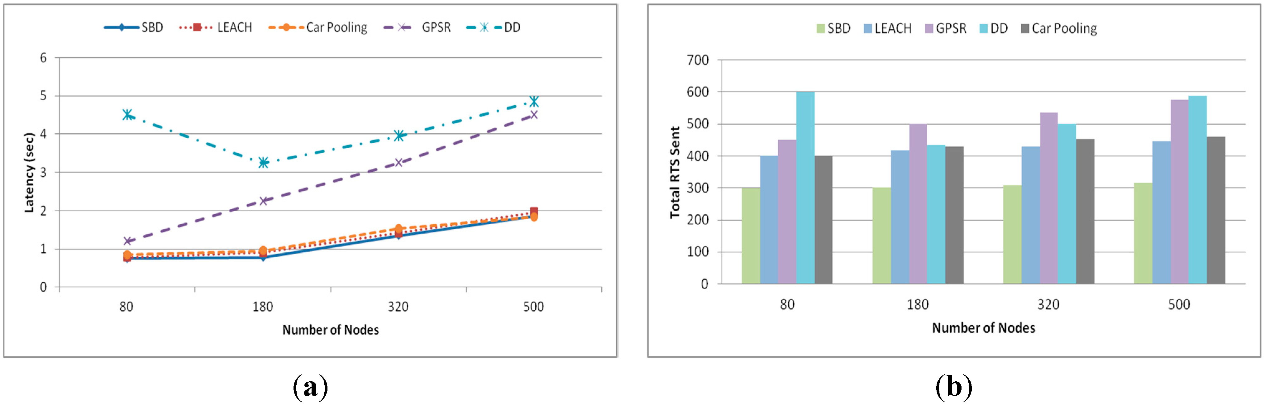
3.4. SBD Routing
In order to relay aggregated packets from
SHk to
SHi, DCSMSS uses the Sector Based Distance (SBD) routing algorithm [
4]. Each round of SBD consists of two phases: (a) Learning phase and (b) Relaying phase. The learning phase is again divided into three stages: (I) Sector head TDMA slot assignment stage using the grid coloring algorithm (GCA); (II) Member-SH association stage; and (III) Intra-sector TDMA slot assignment stage for member nodes managed by the SH
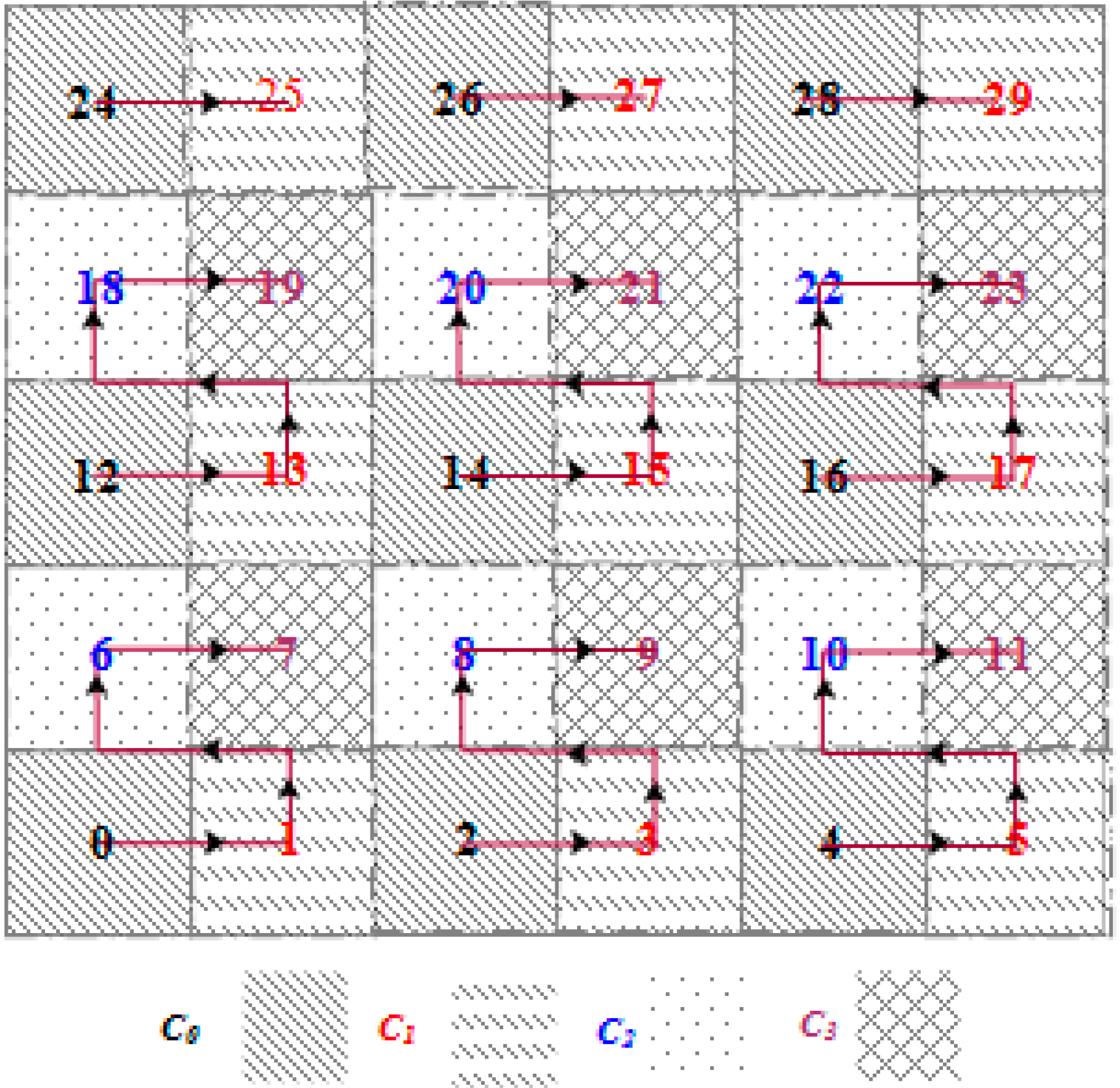
. In the first stage of the learning phase, each SH finds the non-overlapping operating slot for corresponding sectors using Algorithm 2. It is assumed that each SH is configured to be aware of the number of sectors in the deployment layout. Using Algorithm 2, all sectors of any grid size could be assigned with conflict-free TDMA slot by reusing only four time slots. For example, Algorithm 2 has been applied to a grid of 30 sectors (see
Figure 4). Each sector of the grid is assigned with conflict free time slot by reusing only four time slots (
C0~
C3). Sectors with similar time slot can perform concurrently without any interference.
| Algorithm 1. Pivot Point Generation Algorithm (implemented at each SH node). |
Input: attrRangeTable  (containing minimum, maximum, average and theta of each attribute), W (weights to different attributes based on their importance in the event description).
Output: P (derived pivot point for each sector)
1: mapRec.minRange ← 0; mapRec.maxRange ← 0
2: m ← lengthof(attrRangeTable)
3: for each i from 1 to m do
4:	 mapRec.minRange ← mapRec.minRange + (attrRangeTable[i].min/attrRangeTable[i].max) × W[i]
5:	 mapRec.maxRange ← mapRec.maxRange + (attrRangeTable[i].max/attrRangeTable[i].max) × W[i]
6:	 mapRec.com ← mapRec.com + (attrRangeTable[i].avg)/attrRangeTable[i].max) × W[i]
7:	 mapRec.theta ← mapRec.theta + (attrRangeTable.theta)/attrRangeTable[i].max) × W[i]
8:	 i ← i + 1
9: end for
10: comLowerLimit ← mapRec.com − mapRec.theta
11: comUpperLimit ← mapRec.com + mapRec.theta
12: // S is the total number of sectors
13: η ← (comUpperLimit − comLowerLimit)/(S − 1)
14: for each j from 0 to S do
15: 	 if j = 0
16:	   then P[j] ← mapRec.minRange
17:	 else if j = S
18:	   then P[j] ← mapRec.maxRange
19:	 else
20:	   P[j] ← comLowerLimit + j × η
21:	 end if
22:	 j ← j + 1
23: end for
|
Hence, the frame length, denoted by
L, of a round can be defined as:
Here, ∆t is the length of the TDMA time slot assigned to each sector.
Figure 4.
Slot assignment using algorithm 2 (GCA).
Figure 4.
Slot assignment using algorithm 2 (GCA).
| Algorithm 2. Conflict free TDMA frame slot assignment GCA (implemented at each SH node). |
Input: HD = 2 (circular hop distance between two sectors), m, n (total number of tracks (or rows) and sectors (or columns) in the grid, respectively)
Output: Conflict-free time-slot (Ci) with frame length L = 4 × epoch (length of the slot assigned to a sector)
1:      for each j from 1 to m do
2:        for each i from (j − 1) × n to (j × n − 1) do
3:          if i < n × j
4:           then SHi ← C0
5:          end if
6:          if i +1 < n × j
7:           then SHi+1 ← C1
8:          end if
9:          if i + n < m × n
10:         then SHi+n ← C2
11:        end if
12:        if i + n + 1 < m × n
13:         then SHi+n+1 ← C3
14:        end if
15:        i = i + HD
16:      end for
17:      j = j + HD
16:    end for
|
In the Member-SH association stage, SH broadcasts a beacon frame and a member could receive beacon messages from more than one SH. Each member node then sorts the received beacon frames that come from more than one SH node based on Received Signal Strength Indicator (RSSI) into vector ν(SHi, RSSIi), where RSSIi ≥ RSSIi+1. In the presence of channel noise, fading and attenuation, it is not always possible to estimate the closest SH using RSSI only. Hence, in order to accurately find the closest SH, the round trip time (RTT) method has been used as well. According to this method, each Member Node (MN) sends a packet request to all candidate SHs in the list and waits for an immediate acknowledgment. After receiving the acknowledgment the MN calculates the distance of the corresponding SH from time of flight (TOF). It then calculates a ranking number for each candidate SH based on both RSSI and TOF and selects a SH from the candidate list that has highest ranking (see Algorithm 3).
According to this method, the time of flight, referred to as
TTOF is calculated as follows
Here, TRTT = Round Trip Time of Flight. TTCP = Time to Compute Packet.
The distance between two nodes can be calculated as
Here, c = Speed of Light
The Equation (18) can further be rewritten after adding the faultiness as [
13]:
Here, = Error occurs for ranging in a line of sight setting. = Error due to ranging in a non-line of sight environment.
The negative impacts of multipath effects, a big factor, in
can be minimized using an empirical approach [
14]. Uncertainties and noise in the hardware especially jitter effects play a key role in
. Considering the jitter component
TTOF can be calculated as [
15]
In Equations (20) and (21), TOFR = TOF for the request packet. TOFA = TOF for the acknowledgment packet. JtN = jitter caused by the clock of transceiver. JcN = jitter caused by the clock of microcontroller.
The timestamps that are used to calculate the time between sending a request packet and receiving an acknowledge packet contain the jitter values Jt0, Jc0, Jt3 and Jc3. Another two timestamps that are considered in calculating the computation time between receiving a packet and sending the first bit of the ACK packet contain the jitter values Jt1, Jc1, Jt2 and Jc2.
The
MNs then calculate the rank matrix for each candidate
SH as
In Equation (22), MN is the total number of member nodes in Nth sector.
The MNs, then send an association request to the SH, which has the highest rank in its list. This ensures the association of a member node to its closest head node (see Algorithm 3).
| Algorithm 3. Head_Selection (), implemented in member nodes, selects the closest SH based on the rank calculated using Equation (22). |
Input: rank, SHInfo
1:    sort SHInfo in descending order based on rank
2:    create network layer packet joinCntrlPacket
3:     SHD ← pop top element from SHInfo.SHS
4:     set SELF_NET_ADDR as source, SHD as destination and Packet Type = 4 to joinCntrlPacket
5:     //Unicast joining request to the closest head node.
6:     toMacLayer (joinCntrlPacket, SHD)
|
The SHs create a child table listing all the member nodes from which they receive association request. In the third stage of the learning phase, SHs broadcast a packet containing
Ck (0 ≤
k ≤3), ∆
t and an array γ, where γ = {
m1,
m2,
m3, …,
mi} and |γ| =
Mk. In γ,
mi and
i denote the member node ID and index of this member node in the array, respectively. Each member node then calculates the intra-sector transmission slot based on their position in the array γ by:
In Equation (23),
and
MS-ID are the length of the intra-sector TDMA time slot and the node’s self-network address,
i.e., node’s self-ID, respectively. The number of member nodes in a sector varies due to the dynamic nature of the Member-SH association procedure. Hence, the length of an intra-sector
TDMA time slot can be defined by:
In the relaying phase, all member nodes report their buffered or aggregated sensed data to their associated SH during their allocated intra-sector TDMA transmission slot. A SH, after each epoch,
i.e., after collecting data from all member nodes, forwards the mapped event data (according to
Section 3.2) in a multi-hop fashion to the corresponding sector for storage. In this inter-sector communication, SHs continue forwarding their packets to their immediate neighbor SH, which lies on the same row in the virtual grid (
Figure 1a) until the packet reaches the SH that is on the same column as the destination sector. The packet is then forwarded vertically up or down until it reaches the destination (
Figure 1b). The same process of routing is followed for query request and response. A description of the next hop selection process or algorithm during the relaying phase is given in Algorithm 4, which facilitates the selection of next hop in inter-sector communication. SHs continue forwarding their packets to their immediate neighbor in the same track until the packet reaches the same column where the destination sector lies. The packet is then routed vertically up or down until it reaches the destination.
A SH calls Algorithm 4 while acting as either: (I) a relaying node (receives a packet from MAC layer) or (II) a source node (receives packet from application layer).
| Algorithm 4. Search_Next_Hop (SHi), implemented at each sector head node. |
Input: Target SHi, where SHi ∈ [1...S], m- number of tracks (rows) and n- number of sectors per track (columns)
Output: Next Hop SHk, where SHk ∈ [1...S],
1:   //Finding the row and column position of //destination sector head and current head in the //grid
2:   destCol ← SHi%n;
3:   destRow ← SHi/n;
4:   curCol ← nextHopCol ← (SELF_NET_ADDR)%n
5:   curRow ← nextHopRow ← (SELF_NET_ADDR)/n
6:   SHk ← −1
7:    //Moving the packet to the same column where //destination sector lies
8:    if curCol < destcol
9:       /*Move toward right */
10:     then nextHopCol ← nextHopCol + 1
11:   else if curCol > destcol
12:     /*Move toward left */
13:     then nextHopCol ← nextHopCol − 1
14:   //It is in same column so move toward up or down
15:   else if curCol = destCol
16:     then if curRow < destRow
17:       /*Move vertically up*/
18:       then nextHopRow ← nextHopRow + 1
19:     else if curRow > destRow
20:       /*Move vertically down*/
21:       then nextHopRow ← nextHopRow − 1
22:     end if
23:  end if
24:  /*convert to sector number*/
25:  SHk ← nextHopRow × n + nextHopCol
26:  Return SHk
|
Alternate Route
In the case of any primary route failure (first travels toward a track and then a sector), SBD switches to recovery mode of operation. In recovery mode, SHs follow alternate route:
Case 1: Route interruption along
track path
- (a)
The last relay SHR forwards the packet one hop up or down along sector path.
- (b)
SBD returns to its normal mode of operation.
Case 2:
Route interruption along Sector- (a)
The last relay
SHR forwards the packet one hop left or right along the
track path
- (I)
The recipient SHR forwards the packet up or down along sector path
- (b)
SBD returns to its normal mode of operation.
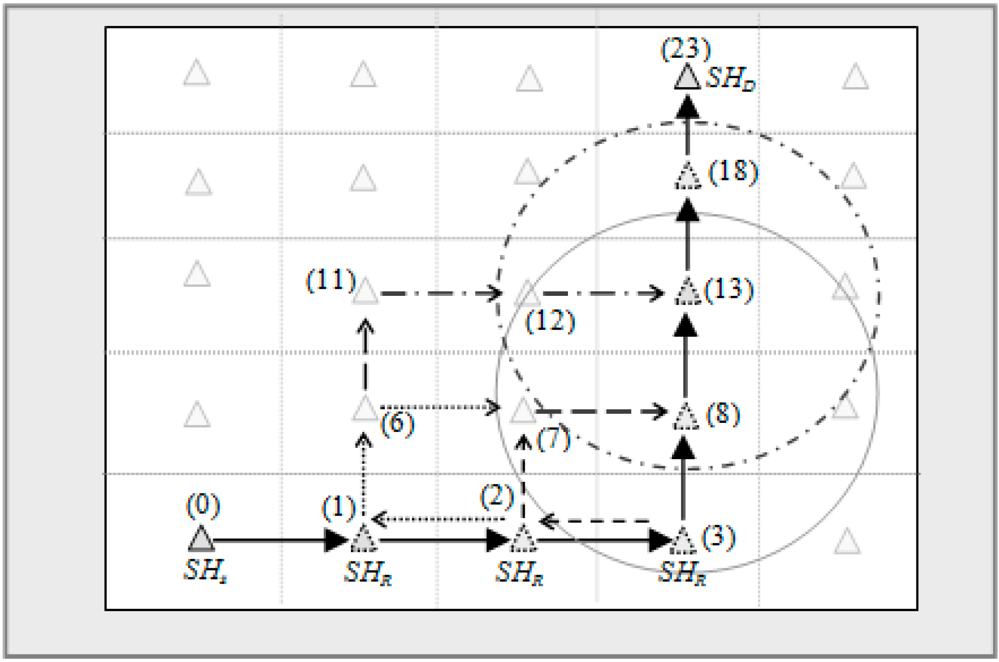
For example,
Figure 5, the source of the packet is
SH0 and destination is
SH23. Hence the primary and possible routes of transmission are:
Figure 5.
Some of the possible alternate routes from SHs → SHD.
Figure 5.
Some of the possible alternate routes from SHs → SHD.
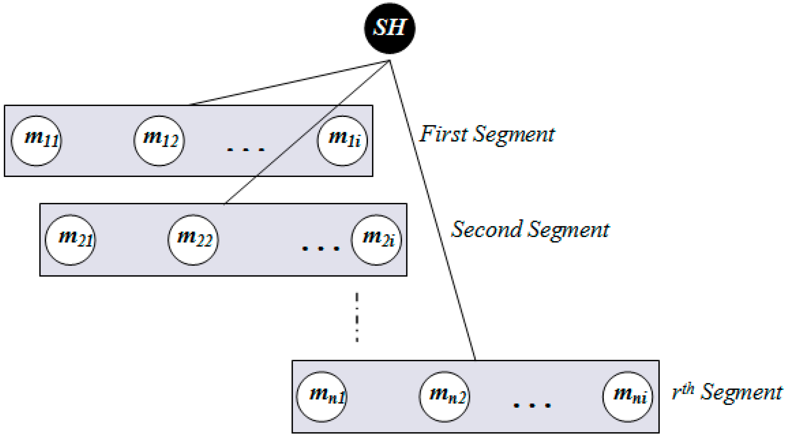
3.5. Insertion
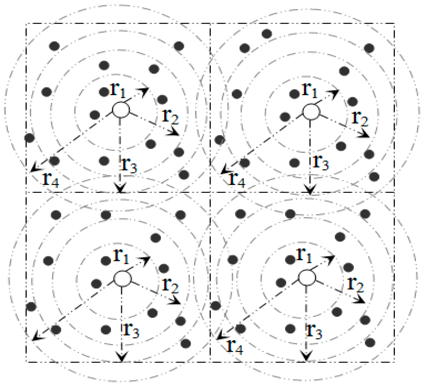
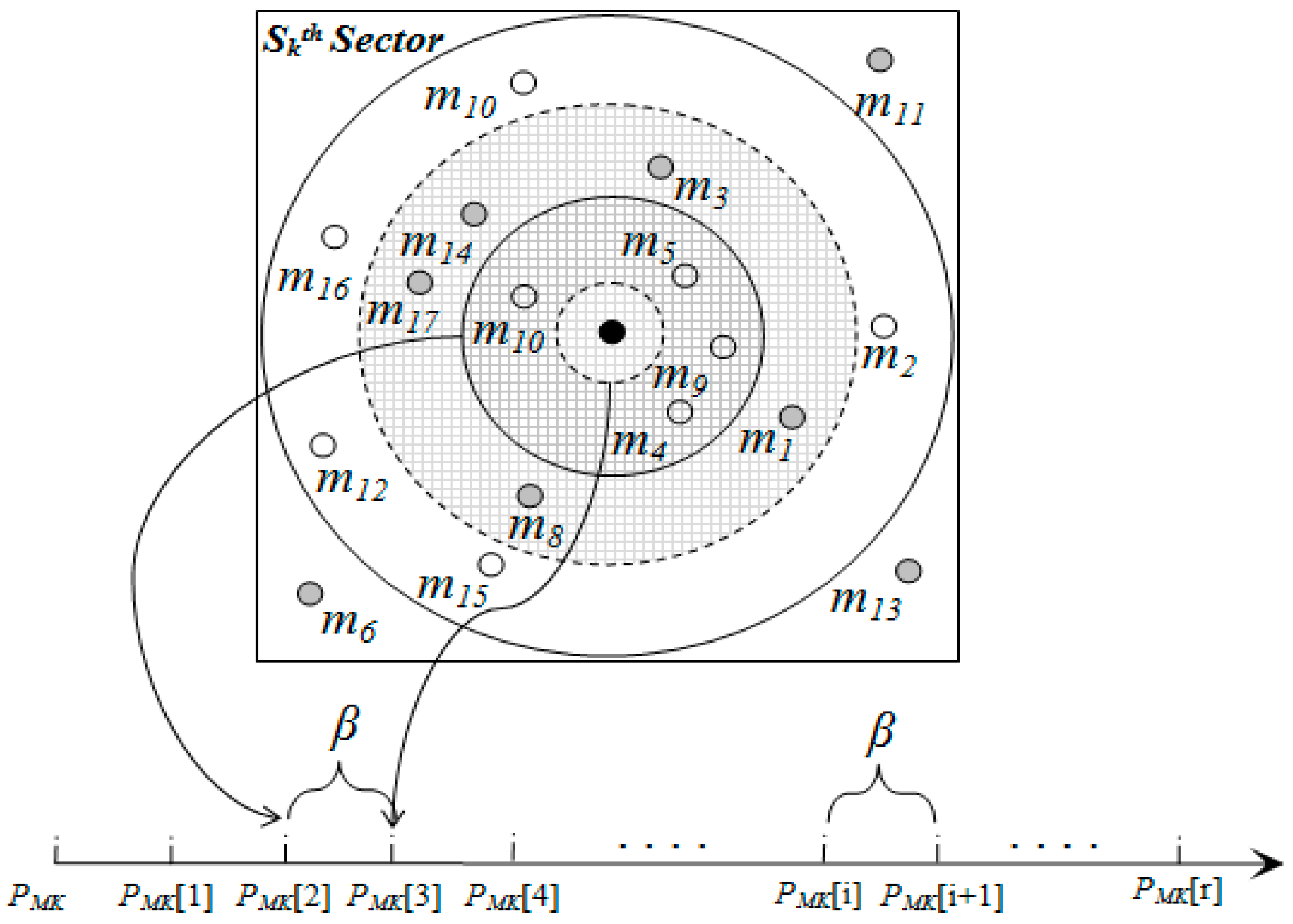
Within a sector, data is further distributed among nodes according to their distance from the SH. To do this, a sector is divided into segments.
Figure 6,
Figure 7 and
Table 4 illustrate the idea of sector segmentation. Given a
kth sector containing
Mk member nodes, the
SHk first sorts all member nodes based on RSSI in ascending order. The member nodes are then divided into
r segments. Each segment forms a ball, denoted by
B(X,Y) (
ri), where the ball centered in (X, Y) of radius
ri. (X, Y) is the geographic co-ordinates for
SHk. The number of segments depends on the WSN application, the size of a sector and the number of member nodes in each sector. Thus the set of sensors that are within a Euclidean distance
ri from (X, Y) form the segment defined by:
Figure 6.
Formation of balls or segments inside a sector.
Figure 6.
Formation of balls or segments inside a sector.
Figure 7.
Segmentation architecture of member nodes inside a sector.
Figure 7.
Segmentation architecture of member nodes inside a sector.
Table 4.
Member table of a SH node.
Table 4.
Member table of a SH node.
![Sensors 15 05474 i002]() |
By Equations (26) and (27), the pivot points for r segments within the kth sector are calculated. An event with hash value, denoted by h, is stored in a member sensor node of ith segment where
. In order to balance the load, data is distributed among the nodes inside a segment in a round robin fashion (see Algorithm 5).
| Algorithm 5. Search_Target_Node (segment[i]), implemented at each SH node. |
  Input: segment[i] (a data structure containing member node ID and tally to count the number of packets stored in the corresponding member node)
  Output: return the target Member Node ID.
  1: sort segment[i] in ascending order based on segment[i].tally
  2: segment[i].tally ← segment[i].tally + 1
  3: memberNodeId ← segment[i].ID
  4: return memberNodeId
|


