1. Introduction
Wireless Sensor Networks (WSNs) are ideal for various scenarios, including environmental monitoring, medical care, military operations, and disaster relief [
1,
2,
3,
4,
5]. In these systems, information relating the location and trajectory (
i.e., localization) of the mobile terminals (MTs) need to be communicated. However, localization is difficult and faces a number of challenges [
6]. Consequently, several methods have been proposed to solve these localization problems. The proposed methods can be broadly divided into two sets of approaches: range-free and range-based approaches. Range-free approaches attempt to localize the position of an MT without relying on the measured distances between target nodes and anchors. Instead, they calculate its position using satellites or some arithmetic according to the sequence of the signal received by the nodes. Examples of range-free approaches include global positioning system localization [
7], the multiple-sequence positioning method [
8], and the regulated signature distance method [
9]. These methods are efficient and accurate in outdoor environments. However, they require costly hardware and are less accurate for indoor environments.
Two types of transmission are dealt with in this paper: line-of-sight (LOS) and non-line-of-sight (NLOS). If there is no obstruction to signal transmission between an MT and a base station (BS), then the transmission is said to be a LOS transmission. On the other hand, in small-scale indoor environments, obstacles such as walls, doors, metal bookcases, and even crowds, can obstruct signal propagation. In such scenarios, the transmission is said to be NLOS transmission. Range-based solutions are more suitable for this kind of environment than range-free solutions. In practical environments, NLOS and LOS transmissions are mixed.
Several range-based techniques have been proposed to reduce the effect of significant NLOS measurement errors. Range-based solutions such as the time of arrival method, time difference of arrival method, and received signal strength indicator method are commonly used to resolve localization issues [
10]. On the basis of measurements obtained from these methods, a variety of mathematical techniques can be used to solve the problems, especially for the NLOS scenario. Kalman filter [
11] works well for linear systems with a Gaussian assumption, whereas for nonlinear systems with a non-Gaussian assumption, the extended Kalman filter (EKF) [
12], the H-infinity filter [
13], and particle filters (PFs) [
14] have been proposed. Of these, PF is a class of recursive Bayesian estimation filters based on sequential Monte Carlo methods. This method divides the area into several grids to form a particle of sufficient density, prior to localization. PF has been proved efficient for models of nonlinear systems and outperforms common nonlinear filters. However, the performance of PF relies heavily on the number of particles and the sequential resampling method. Furthermore, the time required for calculations is inversely proportional to the number of particles selected. Vera
et al. presented the Easy to Deploy Indoor Positioning System [
15], which is able to support the typical localization requirements involved in loosely couple mobile work base on a WIFI system. This method is aimed for fast deployment and real-time operations rather than for location accuracy.
The hidden Markov model (HMM) filter, used extensively in speech processing, is another grid-based method that utilizes Bayesian techniques to estimate the location. In HMM-based localization, a common approach is to use the Viterbi algorithm to calculate position. Morelli
et al. [
16] proposed a Detection/Tracking Algorithm (D/TA) based on this technique and reported satisfactory experimental results. Chen
et al. [
17] proposed an interacting multiple model (IMM) that combines various methods, on the basis of the probability of interaction, to solve the localization problem with satisfactory precision. Performance analysis methods for WSN localization have also been extensively researched. Of these, the Cramér–Rao lower bound (CRLB) is an optimality criterion for the simulation environment.
In this paper, we propose a method that enhances the HMM filter using a modified hidden Markov model (M-HMM). This method determines a compromise solution to improve both efficiency and accuracy. The IMM technique is then used to transform the hidden states between the high-speed and low-speed situations. Thus, it can satisfactorily simulate a real movement environment. Moreover, the IMM is treated as a two-state Markov process to interact with high-velocity and low-velocity models. The CRLB of the environmental simulation is also calculated to determine the accuracy of the algorithm. Simulation results show that our proposed method is closer to the CRLB and superior to conventional methods.
The remainder of this paper is organized as follows:
Section 2 provides a brief overview of the methods that have been proposed for the elimination of NLOS errors.
Section 3 discusses background assumptions made.
Section 4 presents the details of the proposed modified HMM method.
Section 5 presents the integrated algorithm formed by combining IMM and HMM.
Section 6 presents the CRLB of the environment.
Section 7 outlines the simulation experiment conducted and discusses the results obtained. Finally,
Section 8 concludes this paper.
2. Related Work
NLOS identification and mitigation techniques have been extensively researched. Several algorithms that operate by identifying and rejecting data received in NLOS situations and using access points (APs) to calculate the position of an MT in LOS situations have been proposed to solve the NLOS localization problem. Chan
et al. [
18] proposed a method that uses a residual test to identify APs in LOS scenarios and then uses the APs identified to locate the position. Heidari
et al. [
19] proposed definitions for under-detected direct path conditions and direct path conditions, followed by a consequent identification technique that uses binary hypothesis testing and a neural network architecture. Yu
et al. [
20] proposed conducting a hypothesis testing analysis in NLOS environments, which significantly improved the accuracy of position calculation. For unknown parameters in the NLOS error method, Chen [
21] used a residual weighting algorithm to mitigate the effects of NLOS error. Marano
et al. [
22,
23] used a support vector machine to solve the problem of nonparametric NLOS identification. On the one hand, this method imposes a formidable computational burden during LOS selection, while on the other hand, it abandons information obtained from the APs in NLOS transmissions. Wang
et al. [
24] presented a data association scheme that incorporates LOS and NLOS range measurement into the PF framework to effect location estimation.
The localization performance of algorithms depends on the NLOS model used. Most NLOS algorithms assume that NLOS error takes the form of a Gaussian distribution. However, in real environments, the distribution of NLOS error is uncertain. Merino [
25] and Wang [
26] used the Gaussian Mixtures Model to solve the problem. McGuire
et al. [
27] proposed a nonparametric kernel method to calculate the propagation delay. Morelli
et al. [
16] proposed an HMM-based method that relies on high-resolution ultra-wideband (UWB) technology. This grid-based approach was proposed to jointly track the sequence of the positions and sight conditions of the MT. The HMM method does not rely on linearization and the Gaussian assumption, which is the hypothesis regarding noise background in most algorithms. Furthermore, in simulations, an exponential distribution is assumed for NLOS. Considering the large computational burden of the HMM algorithm, Nicoli
et al. proposed a jump Markov particle filter approach to locate the positions [
28]. This method is more efficient than that of Morelli
et al. [
16] while exhibiting a similar accuracy to it. In this paper, we propose a modified localization algorithm based on the HMM method that can utilize more information than that of Morelli
et al. [
16] and Nicoli
et al. [
28] regarding the signal received.
Although the above algorithms all exhibit robustness, each algorithm has another specific advantage in particular conditions. Consequently, several of these algorithms have been combined into dynamic systems using IMM. Liao
et al. [
29] proposed a Kalman-based IMM smoother that fuses LOS and NLOS conditions in cellular networks based on TOA measurements. Subsequently, Chen
et al. [
17] proposed an extended Kalman-based interacting multiple mode (EK-IMM) smoother and a fuzzy-based interacting multiple mode smoother [
30] for mobile localization in order to estimate LOS/NLOS transition based on data fusion with TOA and received signal strength (RSS) measurement data. However, they assumed the mobile terminal to have a constant velocity in both methods, which affects the adaptability of the algorithm. Hammes
et al. [
31] combined the EKF in LOS and the robust EKF in NLOS with IMM. Cheng
et al. [
13] integrated the Kalman filter with the H-infinity filter in IMM to improve range measurement. Compared with the algorithm proposed by Hammes
et al. [
31], Cheng used a different arithmetic to solve problems in different situations.
In the methods proposed above, IMM is used extensively to integrate the LOS and NLOS states. However, both the LOS and NLOS information are already considered in the HMM localization model in this paper. Consequently, there is no need to switch modes between LOS and NLOS. Furthermore, the static speed model is a weakness of the arithmetic in the HMM model. Consideration of the velocity of the MT is restricted in the indoor environment, and thus we simply divide the speed model into two parts, using the IMM to render the algorithm more robust against random movements.
Several methods have been proposed to analyze the advantages and disadvantages of various algorithms in this context. They include geometric dilution of precision and the CRLB. Qi [
32], Huang [
33], and Yin [
34] analyzed the CRLB in varying noise backgrounds and sight situations. In this paper, we use the method proposed by Huang
et al. [
33] to calculate the CRLB value of our simulated environment.
3. Background Assumptions
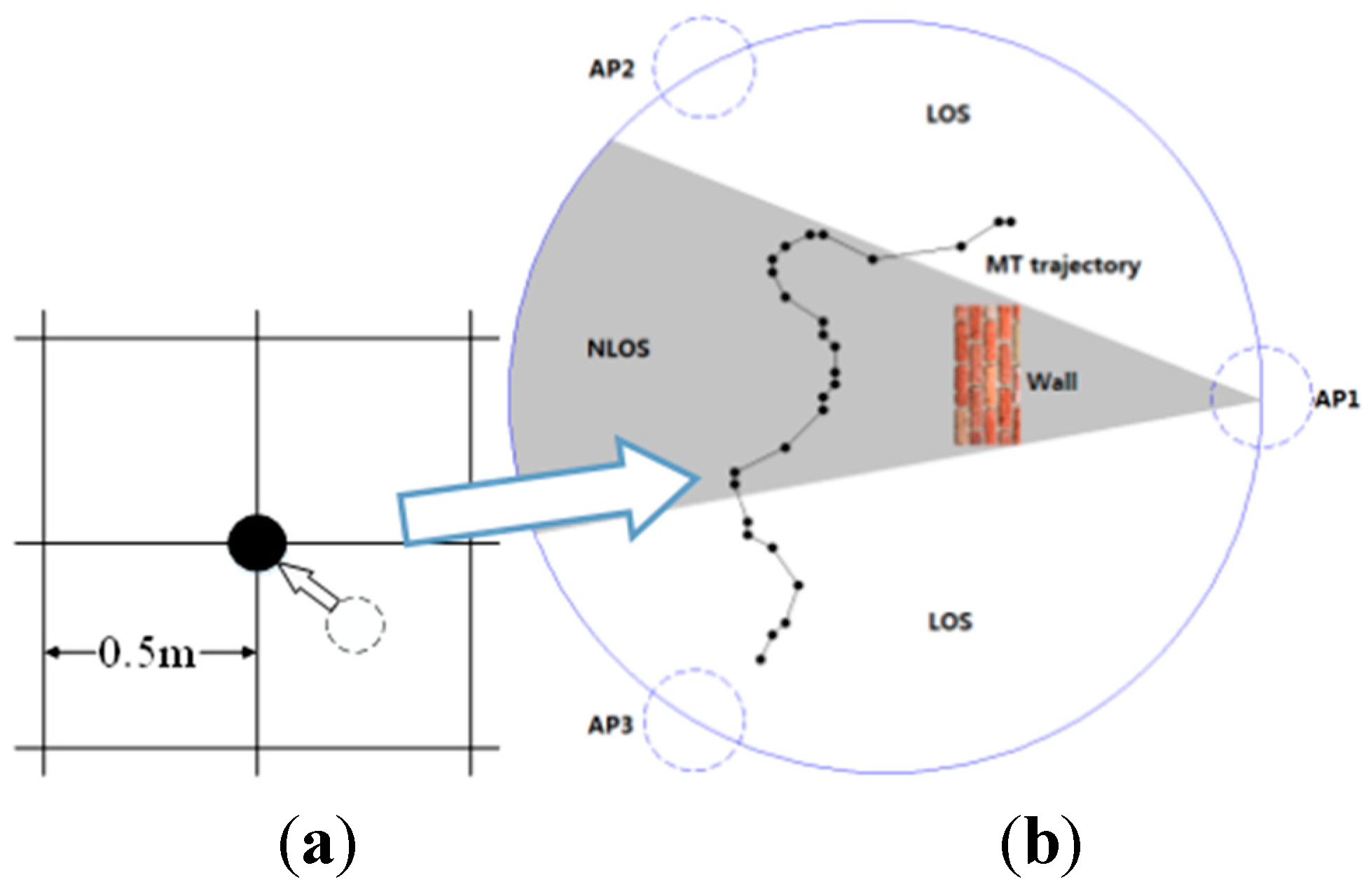
A virtual circular area is first hypothesized as shown in
Figure 1. The MT is then assumed to carry out
k random motions around the particular UWB infrastructure
Q which is defined as the circumscribed circle of three static APs. Its
kth localization position
is calculated by using the signal received from the three
, where
denotes the Cartesian coordinate of the MT in two-dimensional space at the
kth time step. In HMM framework, it is impossible to get the exact sequential Bayesian inference. And as a result, all trajectory points mentioned in this paper are approximated to the nearest grid point that divides the region b, Δ
d = 0.5 m as shown in
Figure 1a. The APs are also assumed to be located on the stationary points, which trisects the circle. Further, if the
lth AP and the MT can communicate without obstructions, as shown by the area in white in
Figure 1b, this situation is defined as an LOS condition and
sl(i) = 0. Conversely, if the path between the AP and the MT is impeded by a thick wall, a metal door, or any other obstacle such that they cannot directly communicate, this situation is known as an NLOS condition, and
sl(i) is assigned a value of one in this case. To simplify this analysis, we assume that each sight condition
sl(i) is independent of position
q(i) and is only related to
sl(i-l). The MT can obtain signal sequence
yi,l from any AP at any time.
Given the above hypothesis, the MT can be localized using knowledge of HMM probability. In the next section, we introduce a signal model and the relationship between the signal model and location probability.
Figure 1.
(a) Discrete approximate schematic diagram; (b) NLOS/LOS condition schematic diagram.
Figure 1.
(a) Discrete approximate schematic diagram; (b) NLOS/LOS condition schematic diagram.
According to Heidari
et al. [
19], the ideal discrete-time description equation for the indoor channel profile is characterized by:
where
e(⋅) represents the time-domain pulse shape of the filter,
Np is the number of multipath components,
represents uncorrelated fading amplitudes, θ represents the phase of the
kth path, and τ
k, including [0,τ
1,τ
2…τ
k-1], is the time delay. We are only concerned with the first arrival delay τ
1, for localization, which is equal to the propagation time given by:
where
sl(i) = 1. for NLOS and
sl(i) = 0 for LOS. According to Morelli
et al., [
35] τ =
d / (
cΔ
t) at any discrete-time τ, and the
lth MT–AP link is defined as two independent real-value zero-mean white Gaussian signals:
where
and
, which is a second-order Gaussian pulse for user
n. To simplify this, we consider only a single-user situation. Morelli
et al. [
16] state that
z ~
N(0,
Cz (τ, Δτ)) is a zero-mean Gaussian vector with covariance matrix
Cz (τ, Δτ). The entire signal
yi,l (
t) is
N(0,
C (τ, Δτ)) with covariance matrix
, where σ
0 is the covariance of the background noise. Moreover
Cz (τ, Δτ), is a diagonal matrix with diag
:
where ρ is the attenuation factor, fixed at 0.9 in this paper, and the receiving power σ
z decreases with increasing propagation distance
d. Note that
.
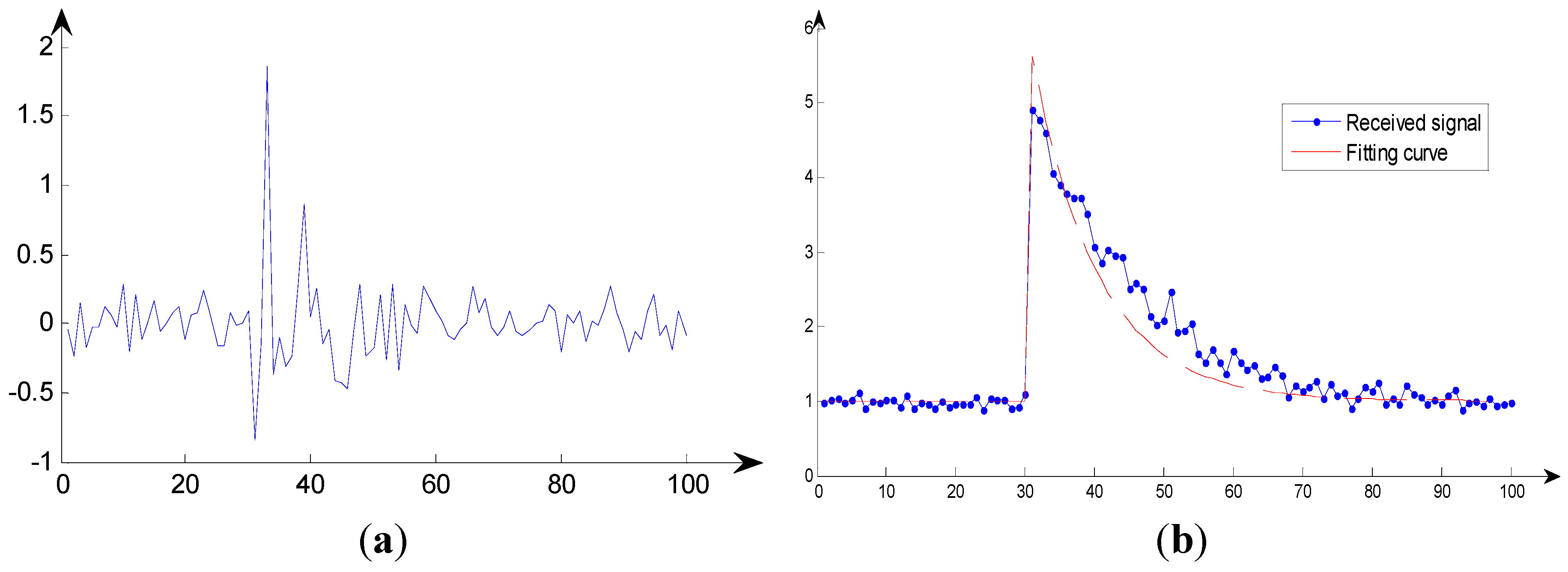
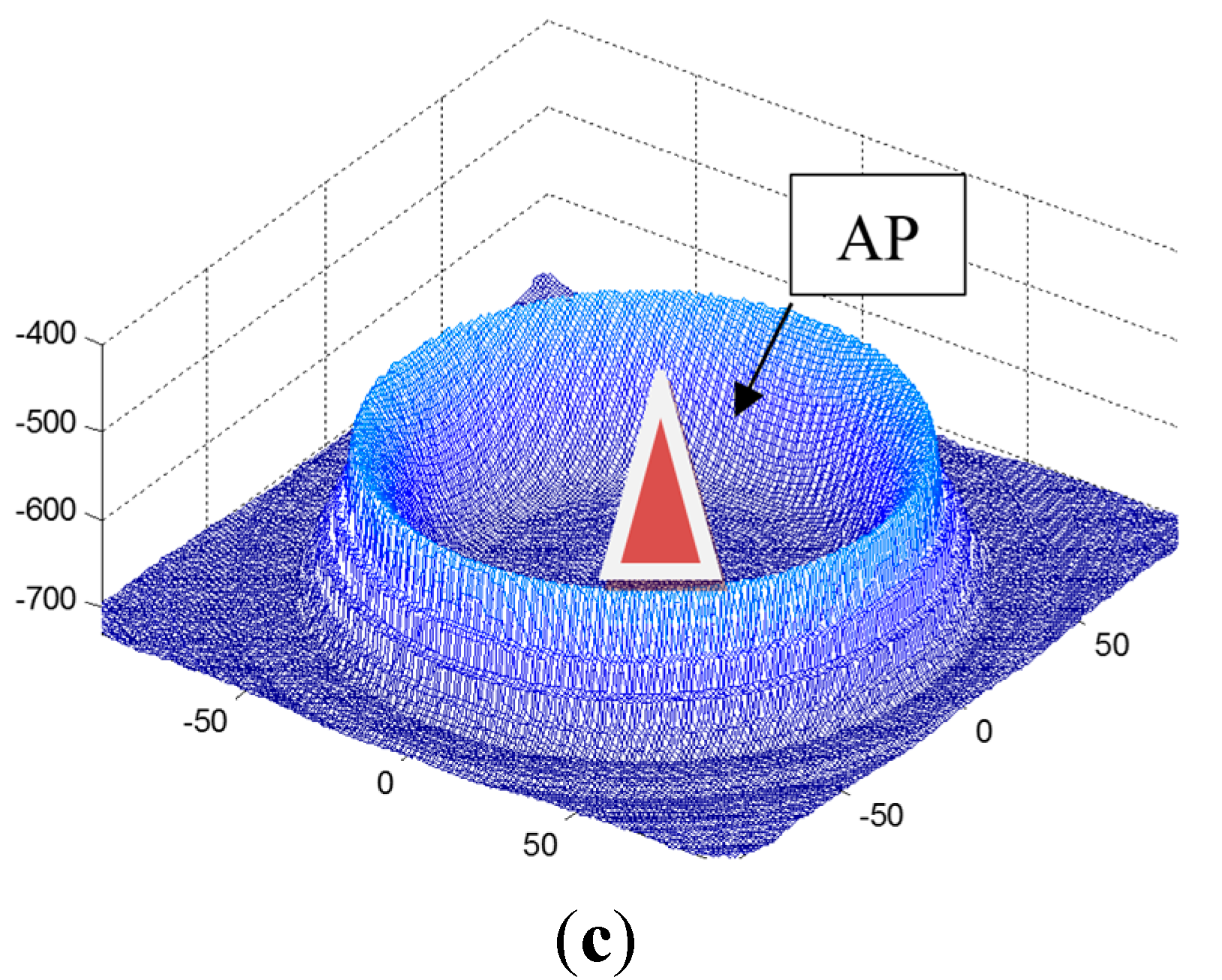
An instance of the value of the measured RSS power is shown in
Figure 2. In the
Figure 2,
.
Figure 2a shows the signal received by the AP at
P disperse times. And in
Figure 2b the solid blue line represents the absolute value of the received signal, and the red dotted line represents the fitting curve of the covariance at each time point.
Figure 2c shows when an AP receives a set of signals, it can estimate the probability of the position of the source by rotating the power delay profile model. In the simulation for HMM, the NLOS delay has an exponential probability density function (PDF)
with σ
δ = 10. In this paper, we assume that the NLOS delay is generated by σ
δ = 7. According to the nonparametric kernel method proposed by McGuire
et al. [
27], the estimated PDF of NLOS delay is as follows:
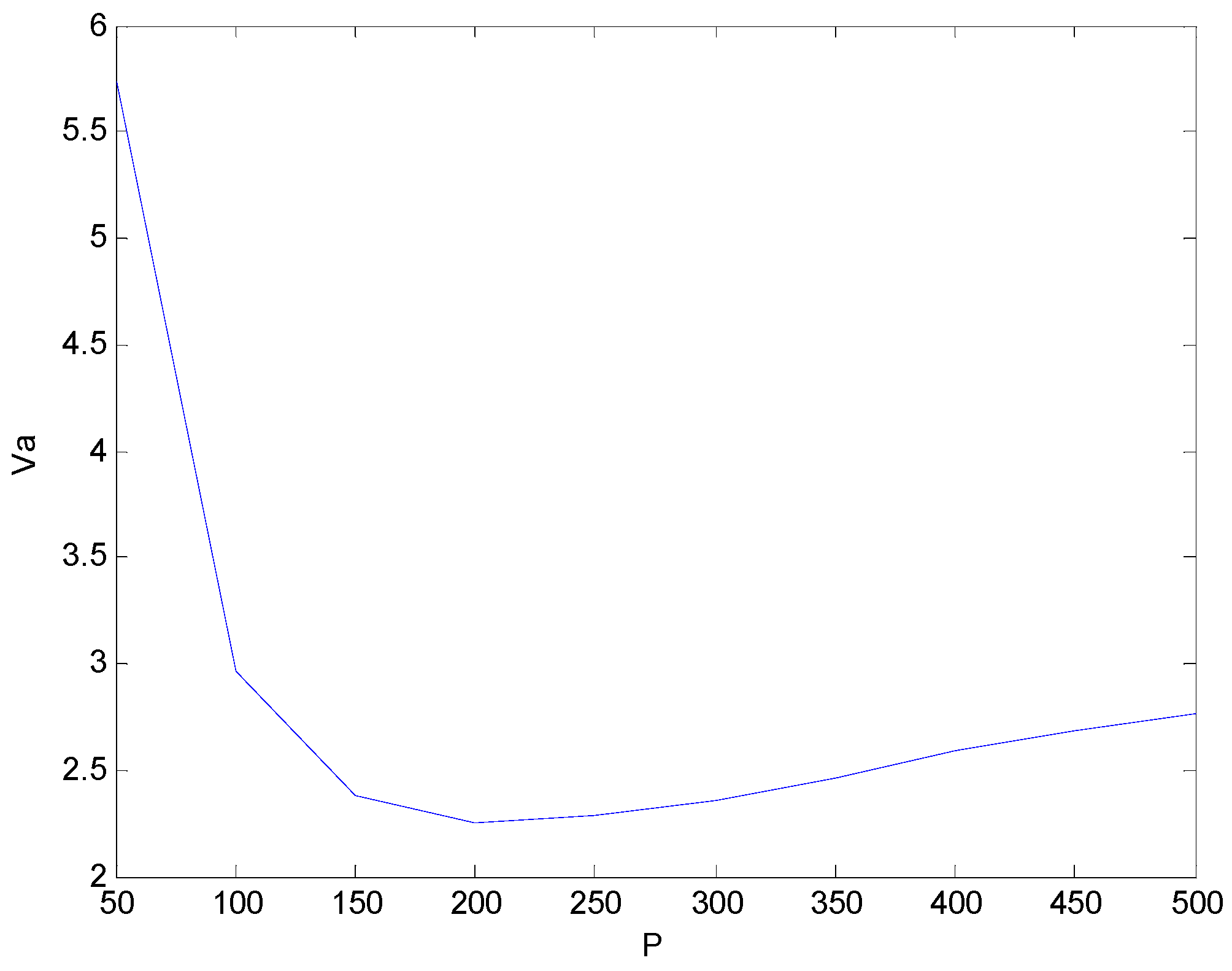
In the above equation, exp(⋅) is a Gaussian kernel function, and
hij is the smoothing constant that determines the width of the kernel function. In this paper, we choose
hij as 0.4 and
P as 200 (
cf. Appendix A). The fitting curve is shown in
Figure 3, with the red line representing the PDF of the Gaussian kernel function and the blue line denoting the PDF of the exponential distribution.
Figure 2.
An instance of the value of the RSS power measured. (a) Example of receive signal; (b) RSS power delay profile model; (c) Example of log-likelihood function for the signal measured by AP.
Figure 2.
An instance of the value of the RSS power measured. (a) Example of receive signal; (b) RSS power delay profile model; (c) Example of log-likelihood function for the signal measured by AP.
Figure 3.
PDF comparison for Gaussian kernel distributions and exponential distributions.
Figure 3.
PDF comparison for Gaussian kernel distributions and exponential distributions.
In traditional localization systems, the basic approach is to estimate the position of the MT through maximum likelihood estimators. As mentioned earlier, the maximum likelihood probability density function of the RSS model, which is the Gaussian probability density function with variables in vector form, is as follows:
As long as MT obtains received signal sequence
Y from the AP, it can calculate the distance probability. On obtaining the distance information from three non-collinear APs, we can calculate the coordinates by executing trilateration or maximum likelihood estimation by merging:
Although this method works well for the LOS case, it has shortcomings. On the one hand, when the MT and AP are in an NLOS situation, significant errors can occur. Further, this method does not consider the regular pattern of motion of the MT, in which the probability of the movement at any moment contains information related to the signal sequence. The HMM algorithm and our proposed improvement on it, described in the next section, solve these problems.
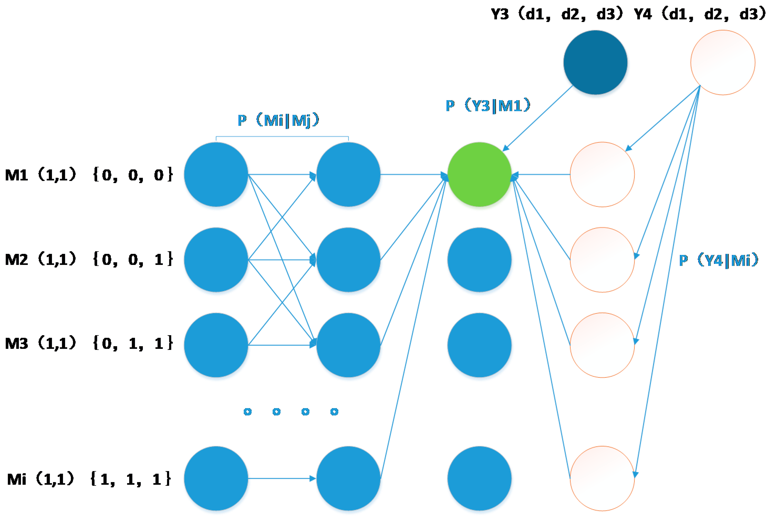
5. Combination of HMM and IMM
In practice, the single transition probability matrix model produces numerous errors because of the variable motion of the MT. This is because each velocity distribution corresponds to a reasonable probability function. Although we can choose a uniform distribution function or other functions, these yield imprecise results. The best approach to solve this problem is to create several separate transition probability models and derive results depending on the velocity distribution in each. The IMM estimator is one of the most effective approaches to this problem in uncertain environmental conditions, where a dynamic system with multiple switching probabilities is used to select the proper transition probability model at the appropriate time.
The MTs in this paper refer to robots or human, and their velocities usually range from 0 to 4 m/s. We thus divide the velocities into low- and high-velocity parts in order to simplify our model. The low-velocity part is a Gaussian function with mean value zero and variance 1.5, and the high-velocity part is one with mean value three and variance 1.5. Note that the narrower the spaces into which we divide the velocity, the more precise the results we obtain. However, our two-part strategy is effective in describing the trajectory of the terminal in this narrow range of velocities.
Figure 9 shows the Markov switching model, which shows that the system varies between the low- and high-velocity models, where
Pab represents the Markov transition probability from mode a to mode b.
Figure 9.
The two models proposed in this paper.
Figure 9.
The two models proposed in this paper.
A schematic diagram of IMM is shown in
Figure 10.
Figure 10.
Flow diagram of the IMM algorithm.
Figure 10.
Flow diagram of the IMM algorithm.
In the figure, U
1(i−1) represents the probability of the presence of the MT in the low-velocity model at time i−1, U
2(i−1) represents the probability of the presence of the MT in the high-velocity model at time i−1, and E(
i) represents the position estimated at time
i, which is the final position. From the figure, we know that the system selects a model based on
and
, which are considered the prior probabilities of each model. It then adds them to the Markov chain and calculates the weight of each model at the final position. The system subsequently calculates the coordinates based on the weighted sum of U
1(
i) and U
2(
i) along with their coordinates
l1(
i) and
l2(
i), respectively. This process can be expressed by the following equations:
In the above equations,
C1 and
C2 represent the normalized coefficients of the low-velocity model and the high-velocity model, respectively;
P1(
mi│
y0:(i+1)) and
P2(
mi│
y0:(i+1)) express
P(
mi│
y0:(i+1)) based on different
P(
Mi│
Mi‒1) models, as described above;
li represents the coordinate information of the MT at time
I; and
q1(i) and
q2(i) represent the positions estimated based on two sequential frames. Finally, the system updates the models and plugs the values of
NP1(
mi│
y0:i) and
NP2(
mi│
y0:i) into each model as the initial values for the next calculation, as illustrated in
Figure 11.
Figure 11.
Updating of weights.
Figure 11.
Updating of weights.
The following equations express the schematic diagram:
where each
NP1(
mi│
y0:i) and
NP2(
mi│
y0:i) is an update for a model used to continue the long-term evolution of the system. And both models are independence. In the next section, we demonstrate the feasibility of our proposed method and its superiority over other methods via simulations.
6. Cramér–Rao Lower Bound on Localization Error in NLOS Environments
The CRLB is a theoretical lower limit for the variance or covariance matrix of any unbiased estimate of an unknown parameter(s). The effects of position precision can be better demonstrated using CRLB, which involves using a nonparametric kernel method to build a probability density function of NLOS errors. The CRLB is also derived in NLOS. In this paper, the arithmetic introduced by Huang
et al. [
33] is used to estimate the value of CRLB related to the deployment of the APs detailed in Section II. The MT with unknown coordinates,
x1y1….
xnyn, and the APs with known coordinates,
, are deployed as described in Section III. The vector of the unknown parameters is
If
is an estimate of θ, the CRLB of this situation can be defined as:
where
is the inverse of the Fisher information matrix (FIM), defined as follows:
where
r represents observation matrix,
Y. The log of the joint conditional PDF is:
Considering that the area of the simulation region is 30 m × 30 m, the limited link capacity, H, is neglected. Furthermore, the positions of the APs are fixed and can be precisely obtained; thus, the information matrix corresponding to the statistics of ranging error in this environment is also neglected. The FIM in CRLB for the case without uncertainty [
33] can then be written as:
Further, the CRLB can be divided into two parts, which can be written as:
where
.
One part of the CRLB is the parameter 1/
A, which is a function containing information on the background noise and the NLOS errors in the environment. Moreover, parameter A can be divided into an LOS part,
ALOS, and an NLOS part,
ANLOS. The relationship between these two parts can be extracted as:
where
pLOS and
pNLOS are the probabilities of the occurrence of the LOS error and the NLOS error, respectively, and should give a total sum of one. Thus, it is clear that when the NLOS error is very small, the value of
ANLOS is close to that of
ALOS and the total value of A is close to that of
ALOS. In this paper, the value of both
pLOS and
pNLOS is estimated to be 0.5 for the simulation environment.
The trace{ } function in Equation (27) above contains information about the system’s geometric distribution. In this paper, the positions of the APs are fixed but those of the MT are randomly generated. For flexibility, we generated 10,000 rational trajectories with 80 steps and calculated their average value. The vector with the value closest to the average value was selected as the most representative trajectory vector to be used as a reference vector.
7. Simulations and Results
In this section, we discuss the simulations conducted to establish the effectiveness of our modified method as well as the precision attained by combining the IMM and HMM using simulation diagrams generated in MATLAB. The PF method proposed by Morelli
et al. [
35] was also used to estimate the equal trajectory in the same signal receiving framework.
We first executed a simulation in a circular environment, as described in Section II (R = 15 m), and set out three APs evenly at the edge of the area. (A robot or a human should actually walk randomly in this area with a terminal communicating with the APs.) We then generated an MT trajectory, as shown in
Figure 6, using Equation (9) with
and σ
v = 3 in 50 iterative steps. The parameters were the same as utilized by Morelli
et al. [
16]: an environment with white Gaussian noise with zero mean and variance σ
02 = 2, path loss with exponent α = 2.4 and ρ = 0.9 and reference distance
dref = 2. An additional NLOS Δτ was created in line with the discrete exponential PDF: σ
d‒1exp(‒
k/σ
d), where σ
d = 7. Sampling frequency
fs = 1 GHz, reference SNR η
ref = 40 dB, channel delay spread τ
rms = 10 ns.
This mathematical model was first used to locate the position for a constant trajectory in order to compare the ML, D/TA, PF, improved [
36], and the modified and replacement algorithms proposed in this paper. The aim is to highlight the improvement in precision by using the modified method
was considered to simplify the analysis and eliminate the data training process. The trajectory was generated as described before. Furthermore, it is worth mentioning that the MT rebounds back into the circle when it “impacts” the edge of the circle, just as light does.
The results for the six algorithms are displayed in
Figure 12.
Figure 12a shows the simulation based on calculations using the ML algorithm,
Figure 12b shows that based on calculations using the D/TA,
Figure 12c represents that using I-D/TA,
Figure 12d shows the results of the simulation based on the PF algorithm, and
Figure 12e,f show simulations based on our proposed modified method and replacement method, respectively.
The blue and the red trajectories in the figures refer to the correct and estimated paths, respectively. From
Figure 12a, we know that the ML estimation contains several false points.
Figure 12b shows that the estimated points show a large disparity with the true trajectory, especially in the determination of the tendency of the MT movement. However, no false points are apparent. This is because the improved
is closer to the real-world situation (
).
Figure 12c shows that the improved algorithm indeed improves the accuracy of localization, whereas
Figure 12d shows that the PF algorithm is similarly accurate to the D/TA algorithm.
Figure 12e shows that the trajectory calculated by the modified algorithm is smoother and more stable, and
Figure 12f shows that the replacement algorithm is more accurate than the M-HMM algorithm.
Figure 12.
Simulation trajectory of various algorithms: (
a) Trajectory estimated by the ML algorithm; (
b) Trajectory estimated by the D/TA estimation in [
16]; (
c) Trajectory according to I-D/TA estimation; (
d) Trajectory estimated by the PF algorithm; (
e) Trajectory estimated by the M-HMM algorithm; (
f) Trajectory using RM-HMM estimation.
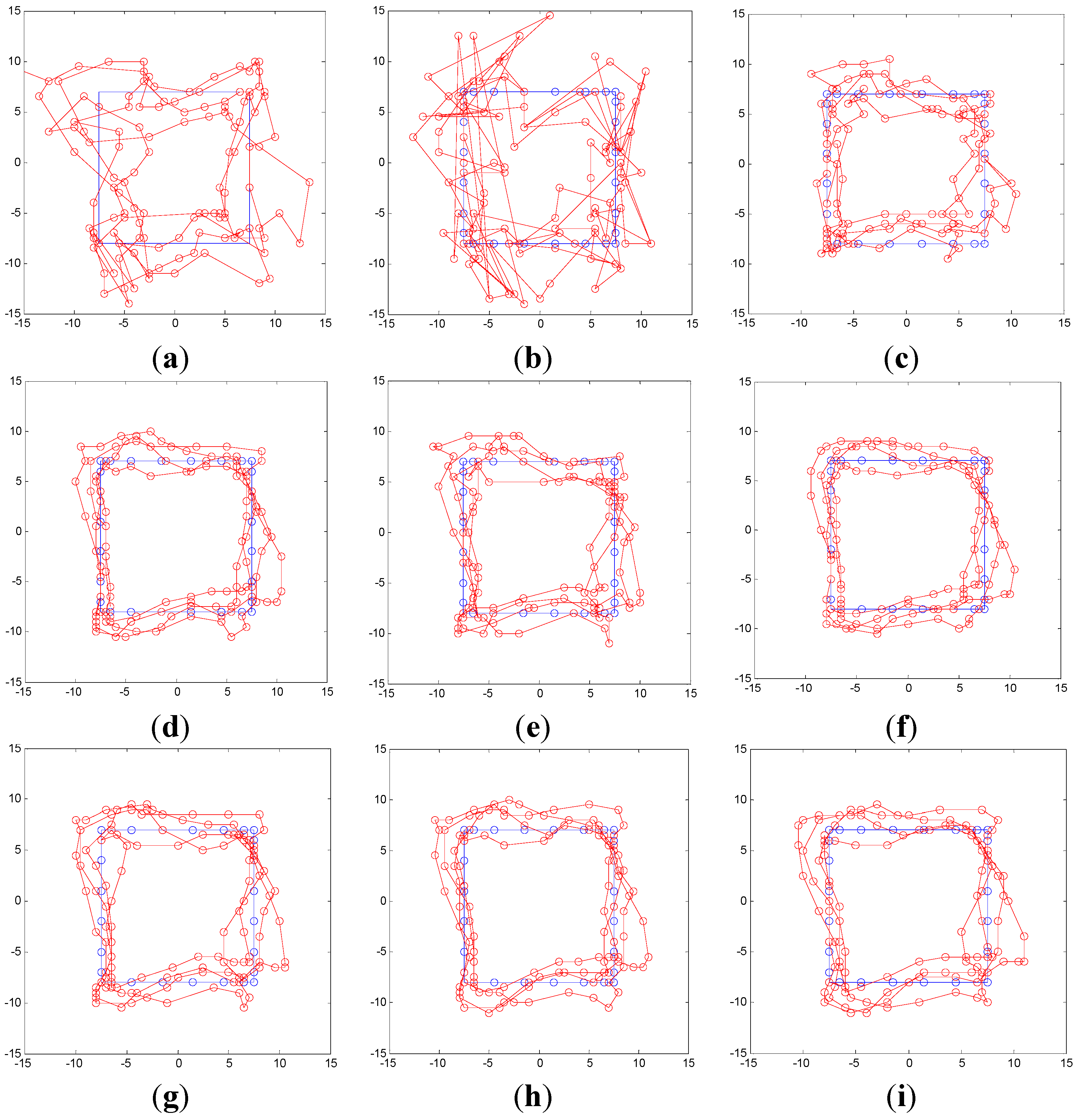
The sight conditions with respect to all APs are represented in
Figure 13, where the blue and white squares represent NLOS and LOS situations, respectively. It is clear that the MT is in an adverse sight condition at the conclusion of the constant trajectory.
Figure 13.
LOS/NLOS situations.
Figure 13.
LOS/NLOS situations.
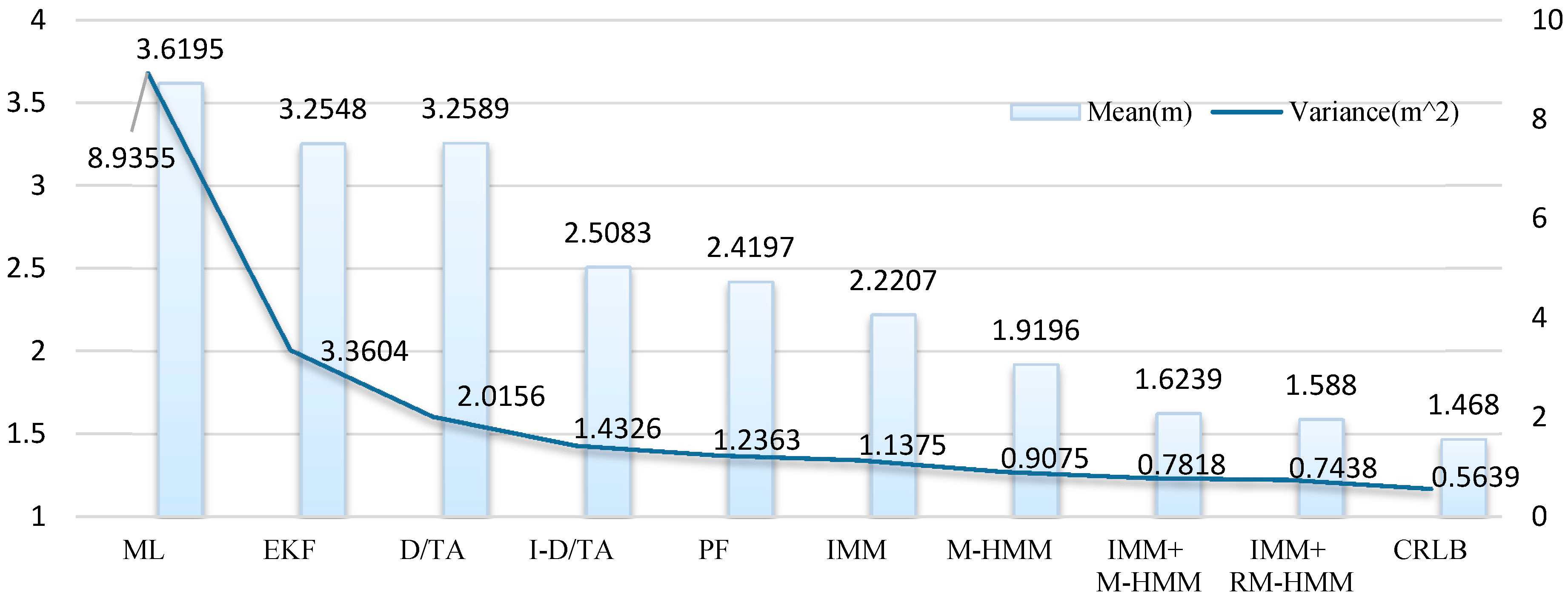
The average error and the variance of the six algorithms are shown in
Figure 14. From the calculated data, it can be seen that I-D/TA has a much greater effect on the simulated trajectory than ML estimation, even though D/TA performs significantly better than the ML algorithm. The PF algorithm exhibits a similar accuracy and stability to that of I-DT/A. In the same manner, M-HMM and RM-HMM show similar accuracy and stability, whereas the RM-D/TA algorithm is the most accurate and stable method.
Figure 14.
Means and variances of the six algorithms.
Figure 14.
Means and variances of the six algorithms.
In order to better represent the error, a cumulative distribution function (CDF) was plotted for the simulation,
Figure 15. The blue line represents the CDF of the estimation using the ML algorithm, the cyan line represents that of the D/TA, and the red line represents that of the I-D/TA [
36]. The CDF of the PF has accuracy similar to that of the I-D/TA. The RM-HMM and M-HMM also show similar precision, with the former exhibiting the best performance. In
Figure 15, the accuracy of the proposed algorithm can be clearly seen.
Figure 15.
CDF analysis of the six algorithms.
Figure 15.
CDF analysis of the six algorithms.
We calculated the probability
P(
yi│
mi) of the fourth, 14th, 24th, 34th, 39th, and 45th steps to show the transformation from the original algorithm to the improved algorithm. To highlight the improvement, we used contours to represent the probability, with higher probability corresponding to a deeper shade of the relevant color representing it. At every step, the position of the MT was estimated by summing the coordinates and the corresponding
P(
yi│
mi). Consequently, the pattern of the contours can be used to illustrate the precision of the algorithm.
Figure 16a shows the original
P(
yi│
mi) of the I-D/TA, whereas
Figure 16b shows that of M-HMM. It can be seen that the multi-peaks and chaotic peaks obtained in the original algorithm have been reduced in number by M-HMM, which is hence more accurate.
We now describe the use of simulation to establish the effectiveness of the combination of the IMM and the HMM algorithms and compare them with the methods discussed above. We first assumed the new trajectory shown in
Figure 17c. In consideration of the speed of robots and humans, we assumed that the acceleration of the MT was 1 m/s
2 with a maximum velocity of 3 m/s.
Figure 16.
Analysis of five dispersion points based on P(yi│mi).
Figure 16.
Analysis of five dispersion points based on P(yi│mi).
P(
Yi│
M(i)) Further, in view of the building corners, the steering angle at every corner was assumed to be a right angle, which is, in practice, a difficult situation. The MT moved around the square four times (
i = 128). It began at (−7.5 m, −8 m), moved to the right, accelerated uniformly, slowed, and then swerved for each turn. The dispersal motion model is as follows:
where
i represents discrete time and
Vtop = 3 m/s, a = 1 m/s
2,
V0 = 0 m/s, and
n is iterated from zero to seven. A value of n = 0 signifies that the MT is at a bend or turn; in this case,
Vn is 0 m/s, which means that the MT stops once at every corner. The MT iterated 17 times through the trajectory. The high-speed model was chosen to be a Gaussian function with an average value of three and a variance of 1.5, as shown in
Figure 17a. The low-speed model was selected to be a Gaussian function with an average value of zero and variance of 1.5, as shown in
Figure 17b. The values of the parameters of the model were empirically determined.
Figure 17.
PDFs of the high- and low-speed models and the original path.
Figure 17.
PDFs of the high- and low-speed models and the original path.
The simulation results are shown in
Figure 18. The lines represent the same quantities as in Section V-A. The figures compare the true trajectory (blue line) with that calculated (red line) using (a) EKF estimation; (b) ML estimation; (c) D/TA estimation; (d) I-D/TA estimation; (e) PF estimation; (f) M-HMM estimation; (g) IMM + D/TA estimation; (h) IMM + RM − HMM estimation; and (i) IMM + M-HMM estimation. It is clear that ML estimation exhibits the worst performance in localization, whereas IMM + RM-HMM has the best results, which are similar in precision to IMM + M-HMM.
The CDF of each of these seven algorithms are shown in
Figure 19. It is clear that the ML estimation is significantly disturbed, and PF, I-D/TA, and M-HMM show more precise results in increasing order. On this basis, IMM combined I-D/TA and M-HMM. The resulting model further improved the precision of the results, which shows the effectiveness of IMM. It is worth noting that the result obtained from M-HMM is better than that obtained using IMM + I-D/TA. RM-HMM is the best algorithm, and is a modified form of IMM + M-HMM.
Figure 20 shows that accuracy and stability improved every time the algorithm improved. For a single reduction in locating error, I-D/TA exhibits the best performance. EKF performs the best in improving locating stability. Although the improvements resulting from later algorithms are smaller, they improve the accuracy by approximately 10%. In comparison with M-HMM, the accuracy of RM-HMM is closer to that of CRLB.
The IMM state in IMM + M-HMM is shown in
Figure 21. In this paper, the MT interconverts between the low-speed and high-speed situations. To show this operation more intuitively, the probability of the MT occurring in the high-speed mode is shown in
Figure 21 using a blue line with an initial value of 0.2. In the figure, the green background represents the acceleration and deceleration, whereas the yellow background denotes uniform velocity. The red line is a line of reference with probability 0.5. From these data, it can be seen that the probability fluctuates with changing colors, and virtually all the peaks of the blue line match the yellow area, which means that the high-speed model was well selected. On the other hand, the bottom of the blue line matches the green area, which implies that the low-speed model was also well chosen.
Figure 18.
Simulation trajectories of different algorithms. (a) EKF; (b) ML; (c) D/TA; (d) I-D/TA; (e) PF; (f) M-HMM; (g) IMM-D/TA; (h) IMM + RM-HMM; (i) IMM + M-HMM.
Figure 18.
Simulation trajectories of different algorithms. (a) EKF; (b) ML; (c) D/TA; (d) I-D/TA; (e) PF; (f) M-HMM; (g) IMM-D/TA; (h) IMM + RM-HMM; (i) IMM + M-HMM.
Figure 19.
CDF analysis of various algorithms.
Figure 19.
CDF analysis of various algorithms.
Figure 20.
Means and variances of the nine algorithms.
Figure 20.
Means and variances of the nine algorithms.
Figure 21.
Transformation of patterns in the simulation.
Figure 21.
Transformation of patterns in the simulation.
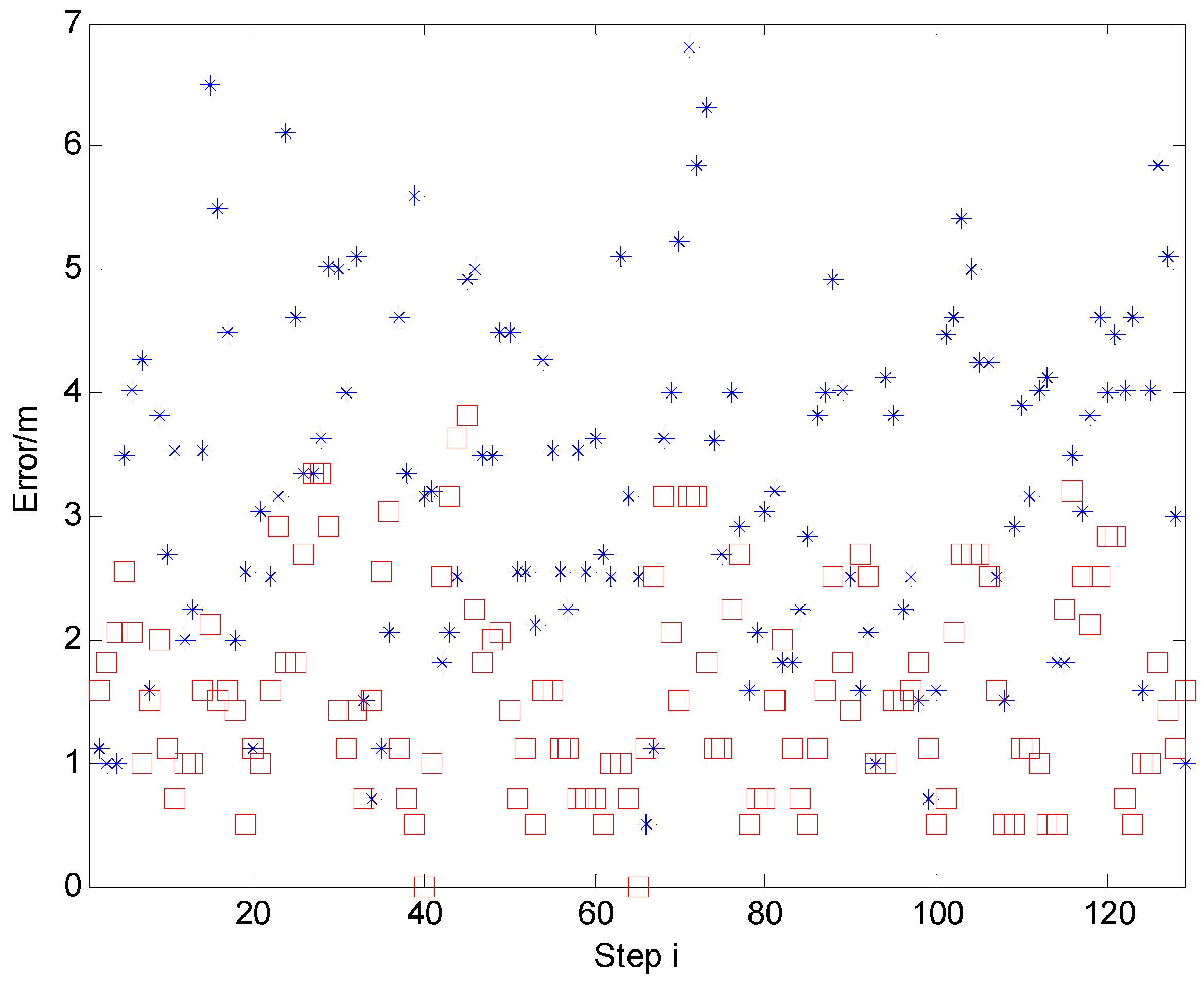
Figure 22.
The error distribution of the improved algorithm.
Figure 22.
The error distribution of the improved algorithm.
Figure 22 shows the error distribution of D/TA and IMM + RM-HMM. The blue star represents the D/TA error and the red square represents the IMM + RM-HMM’s. It can be seen that the algorithm proposed above improves the estimate performance in robustness and precision generally. The analysis of complexity of the algorithms above is shown in
Appendix B.
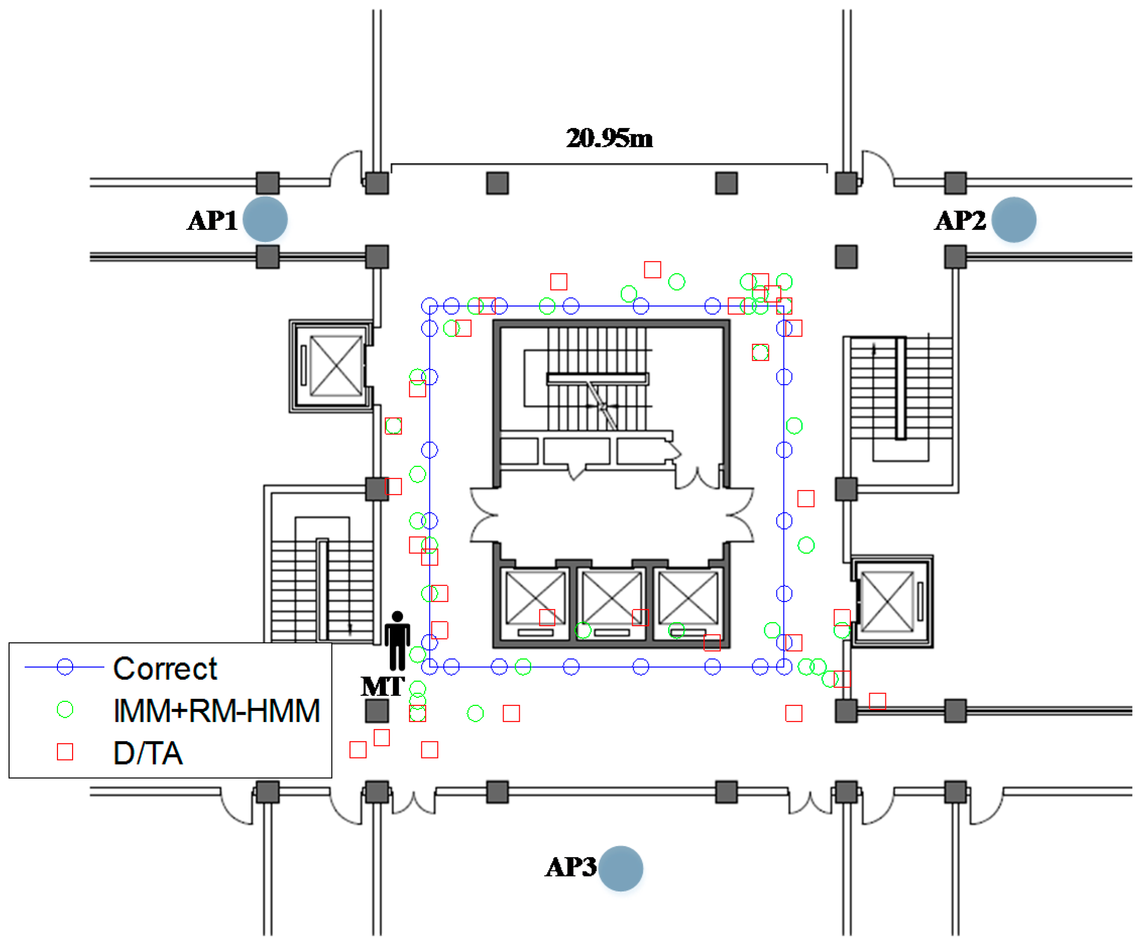
A real experiment is done in the third floor of the Comprehensive Technical Building of Northeastern University to show the effectiveness of the algorithm in complex indoor environments. For comparison purposes, the trajectory of MT is as the same as before, so are the parameters. The AP1 and AP2 are put in the corridor of the building, and the AP3 is put into a room and each AP is bound on a 1.5 meters tall table tripod. Some important signs are put on the ground of the aisle based on the calculation and measurement as shown as blue circle in
Figure 23. A person takes a mobile node walking along the mark points to receive the signal from the three APs. After rounding one lap, the received data are transferred into the computer server with 16 cores and 32GB RAM to estimate the trajectory of MT.
To illustrate the effectiveness of such methods, we set up two experiments in the described scenario and we analyze the results both in simulation and practice environment. The mean value of localization error is found to be 2.73 m in D/TA and 1.69 m in IMM combined with RM-HMM for the simulation respectively. Although the layout of the APs is different from before, the algorithms still show similar precision of localization. In
Figure 23, green circle represents the trajectory of IMM + RM-HMM, and the red square represents the trajectory of D/TA.
Figure 23.
The trajectory of the MT in simulation.
Figure 23.
The trajectory of the MT in simulation.
The practice experiments trajectory is shown in
Figure 24. The legends are similar to the ones in
Figure 23. The new mean values of localization errors are found to be 3.49 m in D/TA and 2.08 m in IMM combined with RM-HMM for the practice experiments.
As can be verified from the scenario, the presence of five big metallic elevators, several power transformation boxes in the wall and metal bookcases cause severe degradation to the accuracy of the localization system in practice. It is worth mention that these phenomena are not reflected in simulation experiment. As is expected, localization with IMM + RM-HMM results in more accurate and stable locations than D/TA.
Figure 24.
The trajectory of the MT in practice.
Figure 24.
The trajectory of the MT in practice.


