2.2. Flow Simulations
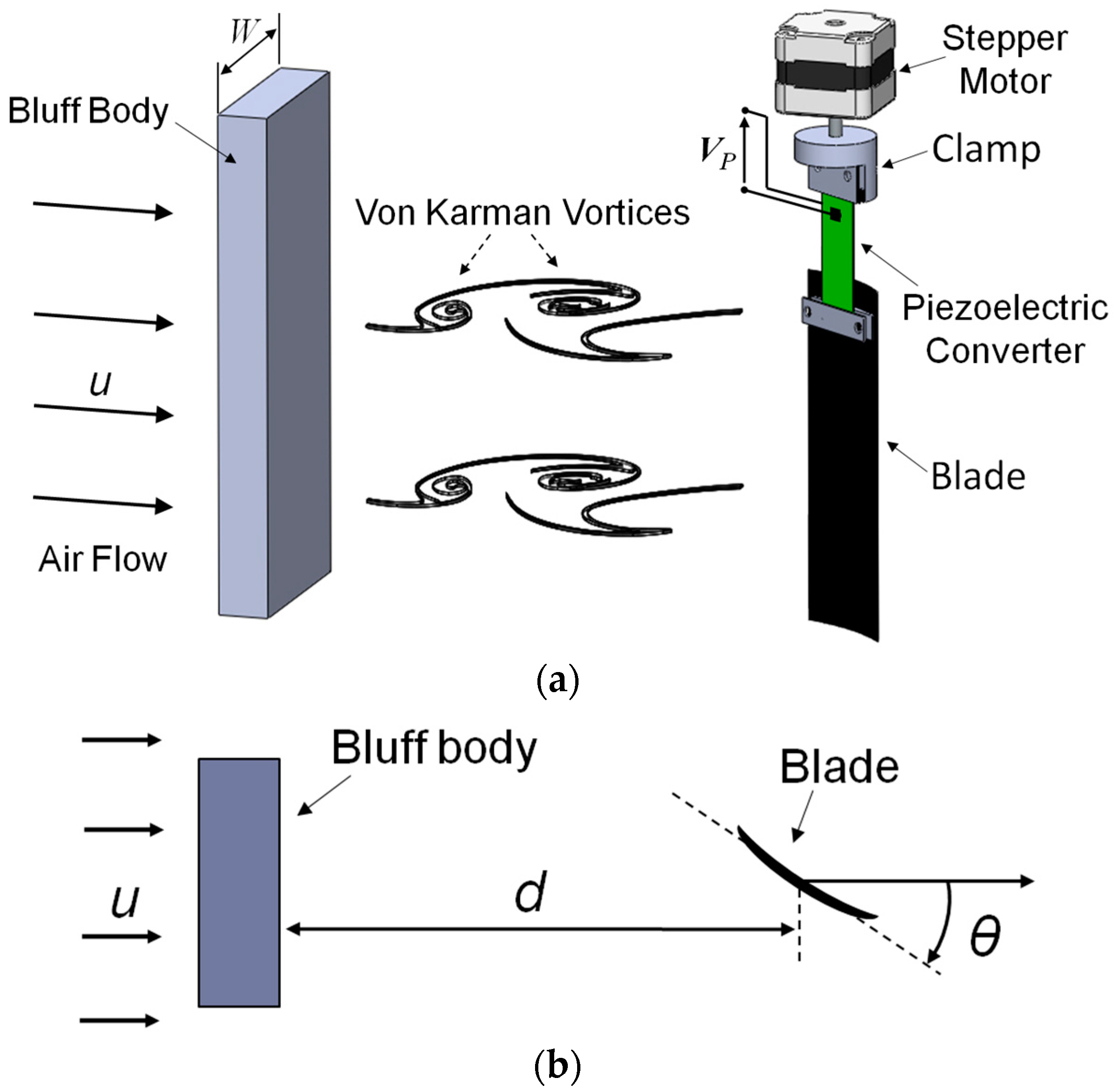
An investigation of the von Karman street behind the proposed bluff body has been performed by Computational Fluid Dynamics (CFD) simulations. Before the subsequent experimental analysis, simulations have been carried out to obtain an estimation of the shedding frequency fu of the vortices as a function of the inlet flow velocity. The simulation analysis was intentionally performed without the beam placed in the flow, since a detailed description of the system with the beam requires a fluid-structure interaction study, which complexity is out of the scope of this paper. Despite the simplified approach, the CFD simulations retain full validity and substantial importance since neither the shedding frequency nor the von Karman street are influenced to a significant extent by the beam presence. Simulations have been performed on the two-dimensional middle horizontal cross-section of the wind tunnel. These simulations are representative of the investigated flow, since the turbulence allows neglecting the effect of the upper and bottom wind tunnel walls, which is confined within the boundary layer.
The large time-step transient solver pimpleFoam of the free software OpenFOAM, version 16.06, has been used to solve an incompressible flow using the k-ε turbulence model. The default model constants available in OpenFOAM have been employed together with the kqRWallFunction and epsilonWallFunction to describe k and ε at walls. The simulated cross-section has a width of 17.5 cm (about 3.5 W) and a length of 62 cm. The bluff body has been placed 25 cm after the inlet section. The inlet flow velocity u has been varied in the range between 2.0 and 7.0 m/s, which corresponds to the actual working condition of the wind tunnel. The frequency of the vortices has been calculated from the time evolution of the simulated velocity field observed at 90 mm downstream from the bluff body.
A grid refinement analysis has been performed to assess the convergence of the simulation results. The vortex shedding frequency
fu has been adopted as the reference quantity to assess the grid convergence. The Grid Convergence Index (GCI) method, proposed by Roache [
19], has been adopted. Three different structured grids have been employed: the coarsest one has a grid spacing of
h3 = 4 mm, and the refinement ratio
r =
h3/
h2 =
h2/
h1 =
has been used to obtain a doubling of the cells number between successive grid steps. The maximum Courant number (CFL condition) has been set as unitary in all the simulations and the time step has been computed consequently. The analysis has been carried out for two different inlet flow velocities of 2.0 m/s and 7.0 m/s which respectively represent the minimum and the maximum values. This is because if the grid convergence is observed at the boundaries of the range of interest, then it is ensured within the whole range.
Table 1 reports the vortex frequency
fu computed for the three different grids. From these values the order of convergence
p, the GCI
2,3 between the medium and the coarse grids, and the GCI
1,2 between the fine and the medium grids have been computed; a safety factor of 3 has been employed in computing the GCI, as suggested in [
19]. The last column of
Table 1 reports the relation between the GCIs, adopted to observe if the three checked grids are in the asymptotic range of convergence. Since the order of convergence
p is about 3 and the GCIs report a low uncertainty on both the two couples of grids and the uncertainty is reduced as the grid is refined, then grid convergence is ensured. Moreover, the relation between the GCIs is near unity, which ensures the analyzed grids are within the asymptotic range of convergence. By the grid analysis results, the finest grid
h1 = 2 mm has been adopted to perform all the simulations.
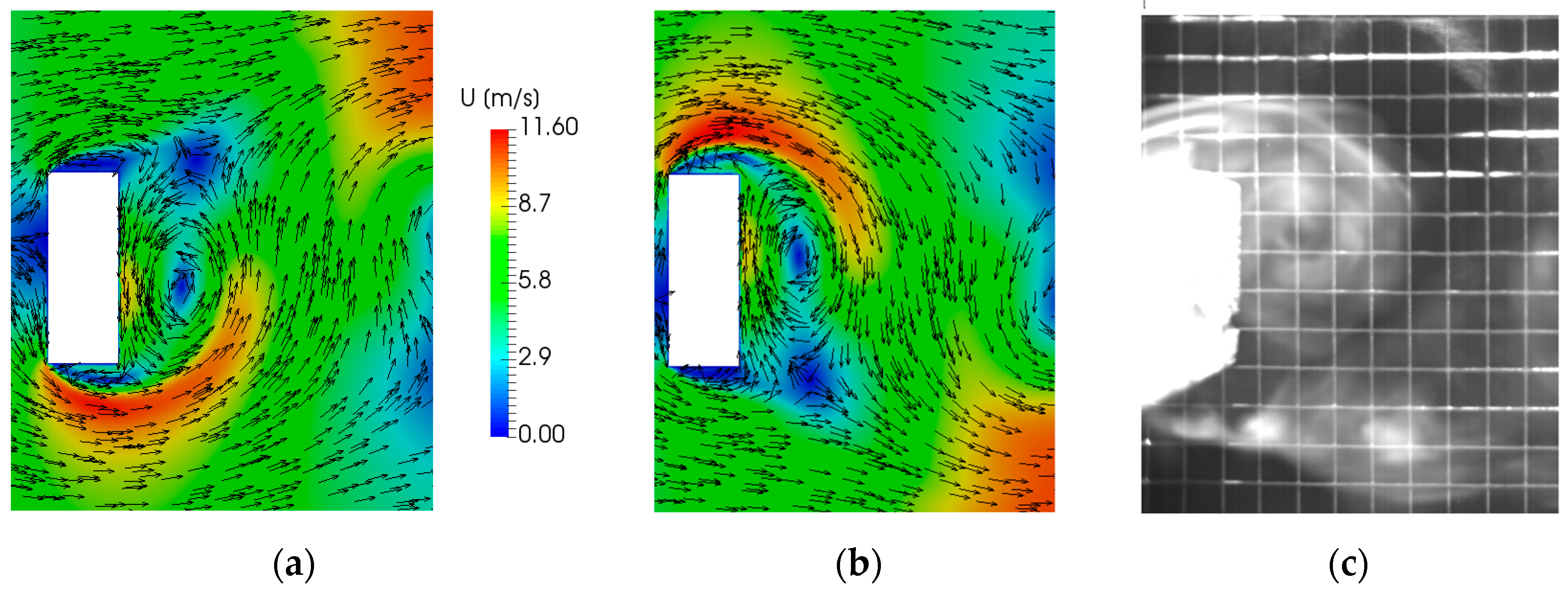
Figure 2a,b show the simulated flow velocity field in the vortex street correspondent to the generation of two subsequent vortices at the left and right edge of the bluff body, respectively. In addition,
Figure 2c shows for comparison the smoke visualization image of the air streamline in the vortex region. A good agreement in the dimension and shape of the vortices can be observed.
The flow in the vortex street consists of a periodic sequence of alternate vortices.
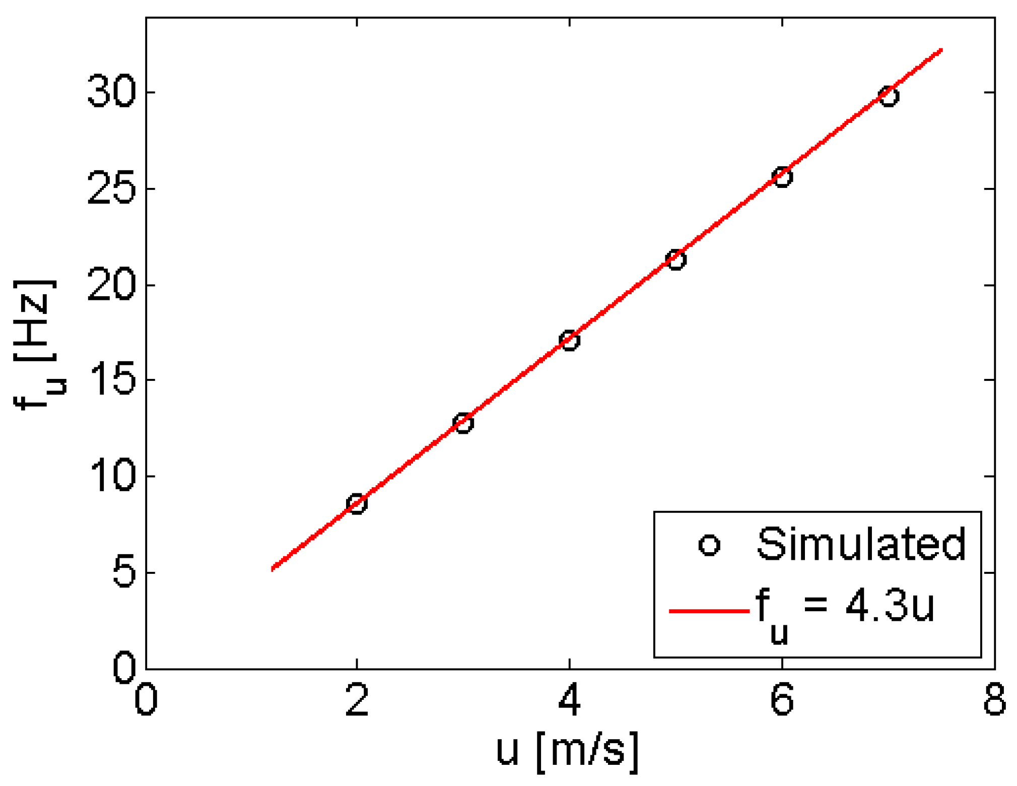
Figure 3 reports the simulated shedding frequency
fu of the vortices, as function of the inlet flow velocity. Results suggest linear relation between
u and
fu, in good agreement with the theoretical expectations since the shedding frequency
fu of the vortices behind a bluff body with a characteristic dimension
W, is linked to the inlet flow velocity
u by:
where
St is the Strouhal number [
10,
12,
15,
20] of the flow. From the linear interpolation of the
fu values, shown in
Figure 3, a Strouhal number
Stsim ≈ 0.23 has been obtained from the CFD simulations.
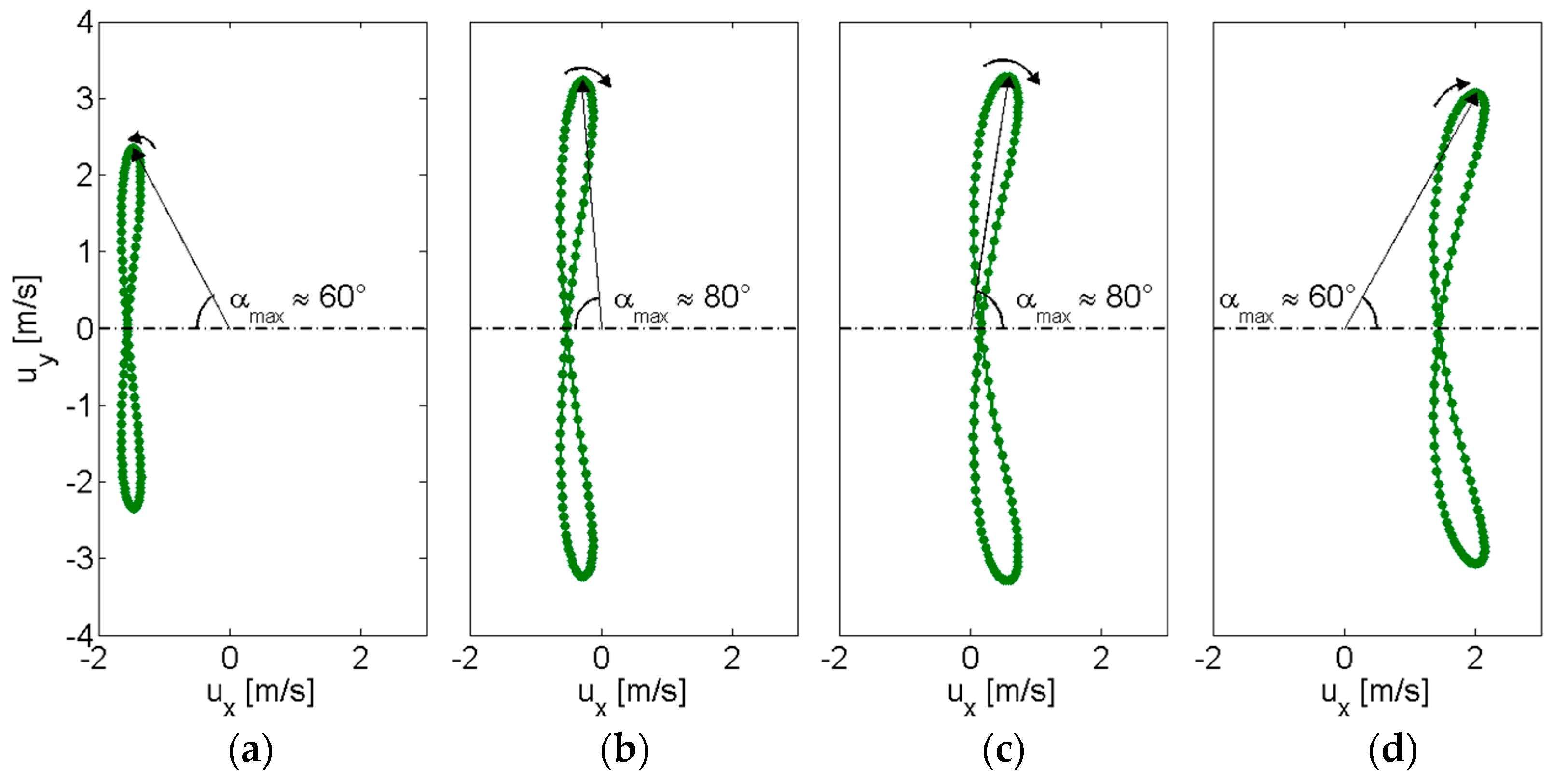
Besides a prediction of the working frequency range of the oscillating beam placed in the vortex street, numerical simulations can provide information on the preferred position behind the bluff body where the beam should be placed. The velocity components,
ux and
uy in the streamwise and spanwise directions, respectively, have been obtained by simulations at different positions behind the bluff body, namely 30, 70, 90, and 130 mm along the central axis. The inlet flow velocity of 5 m/s has been considered in all cases. The plots of
Figure 4 report the loci of the velocity vectors obtained from the components
ux and
uy on the
x-axis and on the
y-axis, respectively, during a cycle composed by two subsequent vortices. Thus, the time evolution of the velocity vector magnitude
and angle α between the central axis and the vector direction can be compared in the four positions.
For the two intermediate distances 70 mm (
Figure 4b), and 90 mm (
Figure 4c), both the velocity magnitude
and the angle α present the maximum variations during the complete cycle, if compared to the other positions 30 mm (
Figure 4a), and 130 mm (
Figure 4d). In fact, together with the maximum variations of α in
Figure 4b,c, which are about −80° < α < +80°, the velocity magnitude spans between 0.5 ÷ 3.3 m/s and 0.1 ÷ 3.4 m/s, respectively. Instead, at short distance behind the bluff body (
Figure 4a), not only the magnitude variation, 1.6 ÷ 2.8 m/s, is lower, but also the same is true for the angle variation, namely about −60° < α < +60°. At this position a recirculation region is present behind the bluff body, as it can be observed by the negative value of
ux. As the distance from the bluff body increases (
Figure 4d, both
and α variations decrease to 1.5 ÷ 3.7 m/s and −60° < α < +60°, respectively, since
ux approaches the inlet flow velocity and
uy reduces because of turbulent dissipation. The results suggest that the distance range between 70 and 90 mm are expected to provide an effective alternate forcing for a vibrating energy harvester due to the best combination between the magnitude variation and the angle variation taking place.
Following these considerations, the beam has been placed at
d = 80 mm ≈ 1.5
W downstream from the bluff body. This choice is supported also by the results reported in [
10], since 1.5
W represents a trade-off between the distance of two times the bluff body width, 2
W, and the distance of two hydraulic diameters of the rectangular section of the bluff body, 1.1
W.
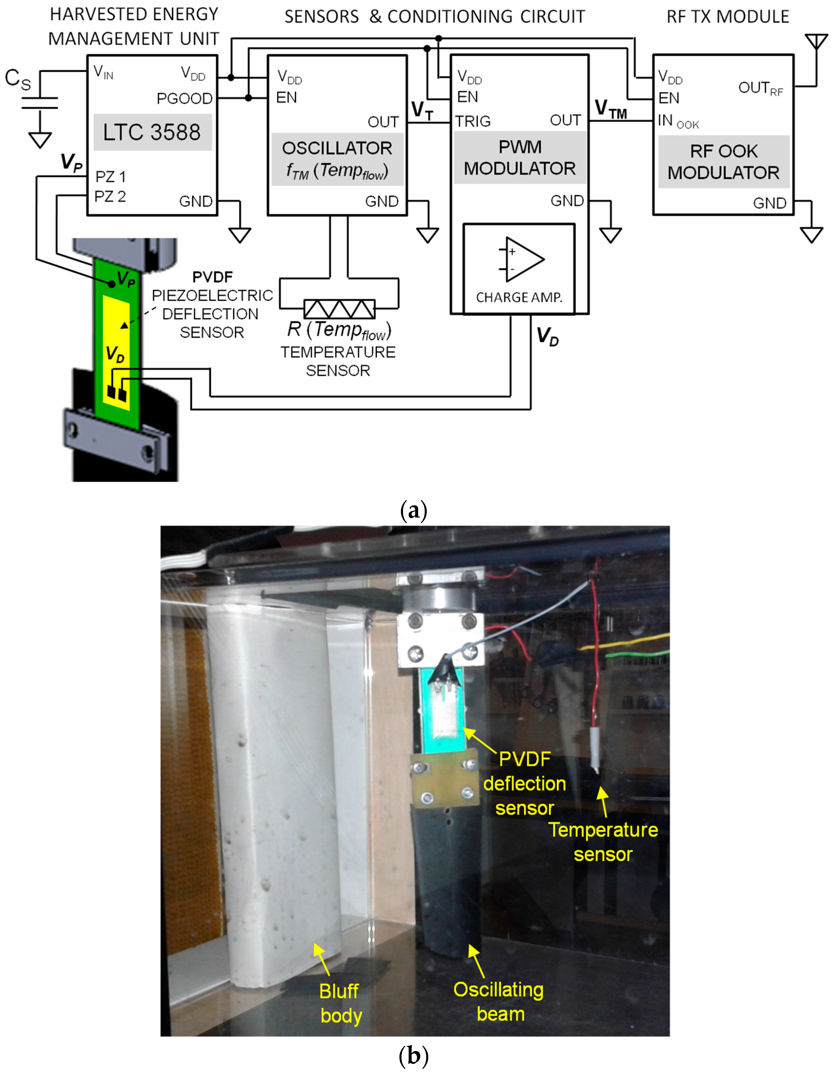
2.3. Experimental Characterization
The converter open-circuit voltage
VP, which is associated to the beam oscillations, has been measured for different beam orientations at three different flow velocities generated in the wind tunnel. The whole range of orientations of 360° has been divided in 200 steps leading to an angle resolution of 1.8°. For each step the voltage
VP has been measured by using an MSO-X 3014A digital oscilloscope (Agilent, Santa Clara, CA, USA) with an input impedance of 10 MΩ in parallel with 15 pF that overall can be assumed as an open circuit load for the adopted piezoelectric converter that has an internal equivalent impedance composed of a capacitance
CP ≈ 305 nF and a parallel resistor
RP ≈ 250 kΩ as measured at 100 Hz by a HP4194 impedance analyzer (Hewlett-Packard, Palo Alto, CA, USA). The flow velocity has been measured by a 405-V1 hot wire anemometer (Testo SE & Co. KGaA, Lenzkirch, Germany) placed before the bluff body in the center of the initial section of the wind tunnel. The sensor has a velocity resolution of 0.1 m/s and an accuracy of ±0.3 m/s. In
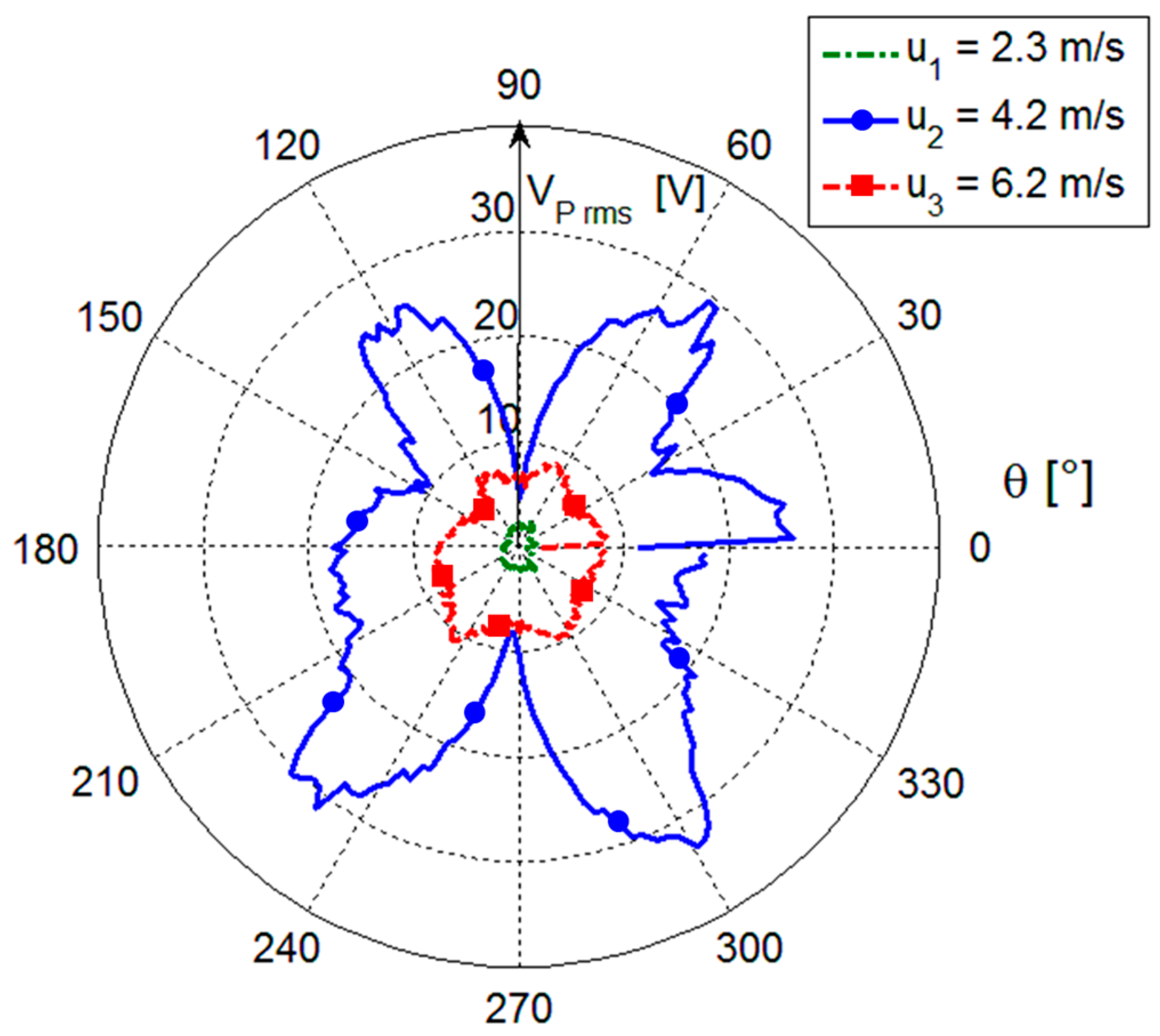
Figure 5 the rms values of
VP measured on a time window of 20 s are shown as a function of the angle
θ for three values of flow velocity, namely
u1 = 2.3 m/s,
u2 = 4.2 m/s and
u3 = 6.2 m/s. As it can be observed, higher rms values are obtained when the orientation angles are about
θ = 60°, 120°, 240° and 300°. This means that, for such orientations, the beam experiences a better coupling with the forcing pressure field. The slight deviations from perfect symmetry in specular orientations of the beam can be ascribed to the asymmetry of the blade profile.
Moreover, in
Figure 5 it can be observed that the highest rms values of
VP, of up to about 30 V, have been achieved for the intermediate velocity
u2, with respect to the values below 10 V obtained for the other velocities. This would seem in contrast with the increasing flow intensity and turbulence with velocity progressively increasing from
u1 to
u3. The reason for the highest rms values of
VP at the intermediate velocity
u2 can be found in the repetition frequency of the vortices that at
u2 becomes close to the resonant frequency
fm of the beam first flexural mode, which is of about 13.6 Hz. As a consequence, under this condition, the vortices excite the beam generating larger oscillations compared to other flow velocities. In particular, this happens for
u3, where, despite the higher velocity compared to
u2, lower rms values are generated.
The effect of the vortex repetition frequency has been investigated by the analysis of the time and frequency behavior of the measured
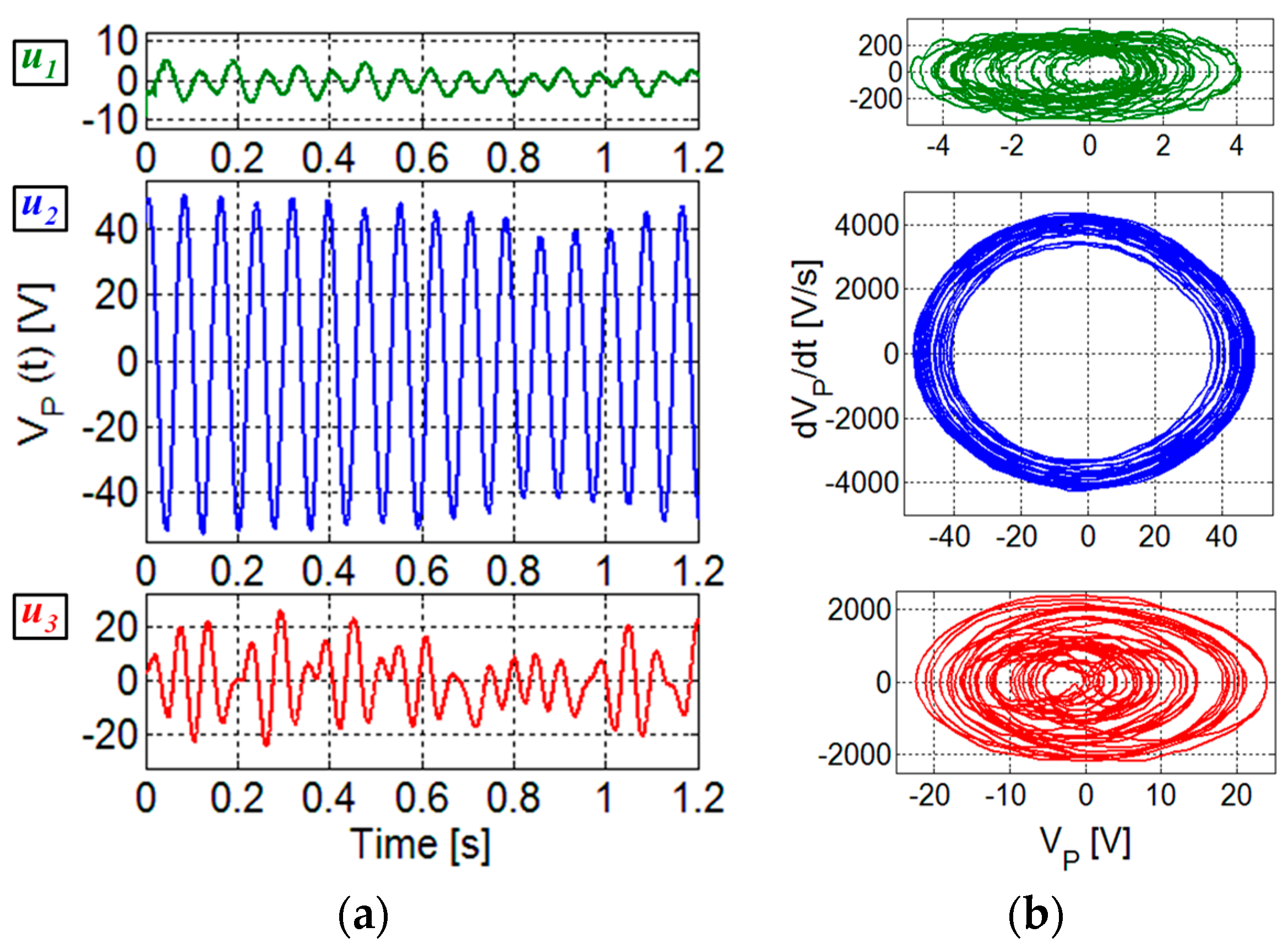
VP at the different flow velocities.
Figure 6a shows the comparison of the voltages
VP versus time for the three velocities
u1,
u2 and
u3, obtained at the fixed orientation of
θ = 300°. This comparison confirms that the higher magnitude of
VP associated to the larger oscillations is obtained for the intermediate velocity, since the repetition frequency of the vortices excites the beam resonance. The trajectories in the phase plane [
21] derived from the time records of
VP are also reported in
Figure 6b. For the piezoelectric element, the open-circuit output voltage
VP and its time derivative d
VP/d
t are proportional to displacement and velocity, respectively [
22]. The comparison of the phase plots show that quasi-periodic oscillations are obtained at
u2, while for
u1 and
u3 sets of manifold trajectories are evident suggesting a more complex dynamical behavior.
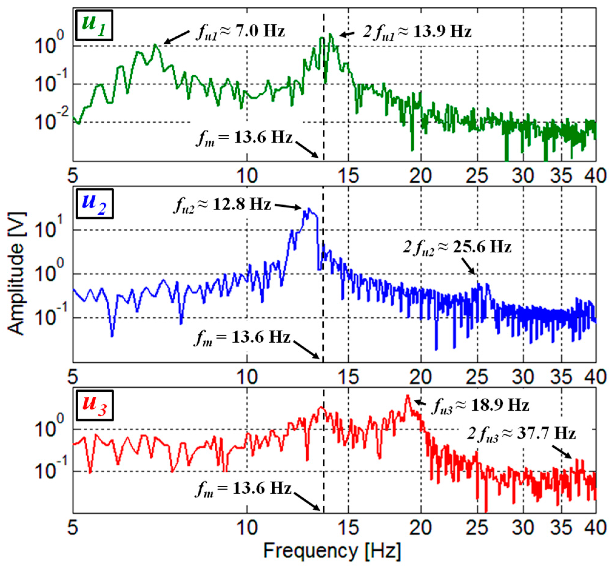
The frequency spectra of the measured voltages
VP have been obtained by FFT processing, considering a time window of 20 s.
Figure 7 shows the comparison among the frequency spectra of
VP measured for the three different velocities considered in
Figure 6. In the spectrum relative to the intermediate velocity
u2, a main component at the corresponding vortex repetition frequency
fu2, well beyond the voltage level at other frequencies, is present. Indeed, at the velocity
u2 it was possible to clearly identify
fu2 = 12.8 Hz since it is near to the beam resonant frequency of 13.6 Hz. From Equation (1) and the frequency
fu2, the Strouhal number of the proposed configuration could thus be determined, resulting in
St ≈ 0.17; this value is in reasonably good agreement with the value of
Stsim ≈ 0.23 obtained by CFD in
Section 2.2.
In this way, Equation (1) also allows to calculate the repetition frequencies
fu1 and
fu3 at
u1 and
u3, resulting in
fu1 = 7.0 Hz and
fu3 = 18.9 Hz, respectively. As it can be observed in
Figure 7, main components in the spectra of
VP for
u1 and
u3 are present at the frequencies
fu1 and
fu3. This confirms that the oscillations contain a frequency contribution at the repetition frequency of the forcing vortices also for the velocities
u1 and
u3. In addition, it can be observed that in all three spectra components are also present at the second harmonics of the repetition frequencies.
Given the sufficiently high bending stiffness of the piezoelectric element, no significant departure from mechanical linearity is expected in the explored flow range. This is confirmed in
Figure 6a where the output voltage
VP is shown to be essentially a sinusoid when the system is excited at a vortex repetition frequency close to the resonant frequency
fm, i.e., for velocity
u2. Then an analysis of the frequency spectra in linear conditions is appropriate.
For this purpose, it can be assumed that the action of a vortex on the beam consists of a force pulse and that the oscillation of the beam caused by the force pulse is a sinusoidal damped oscillation. Thus, when the oscillation is generated by a periodic sequence of vortices with a repetition frequency
fV, the voltage
VC(
t) at the output of the piezoelectric cantilever, can be expressed as the sum of sinusoidal damped oscillations:
where
s(t) represents the step function, and
Tv = 1/
fv is the time interval between two subsequent vortices, and
k is an integer. The parameters
Ad,
αd and
fd represent, respectively, the amplitude, damping factor and oscillation frequency of the damped oscillation of the beam due to an applied force pulse.
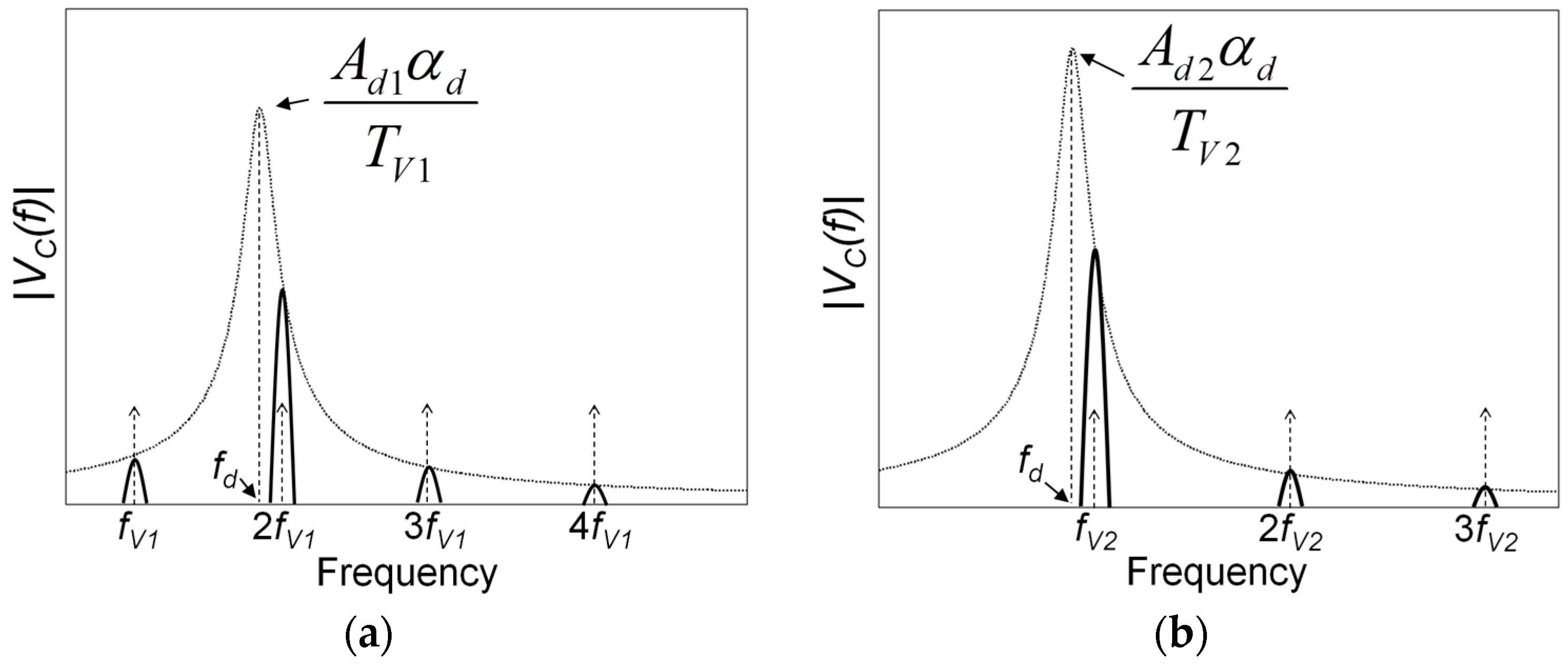
The frequency spectrum
VC(f) can be derived by the Fourier transform of the time function in Equation (2) as follows:
The spectrum
VC(f) consists of the product of two terms, where the first term represents the spectrum of a single damped oscillation of the beam centered at its damped frequency
fd, and the second term
δfv(f) consists of a sequence of Dirac pulses equally spaced of
fv. A graphical representation of the magnitude of
VC(f), derived from Equation (3), is shown in
Figure 8.
The comparison between the spectra of the measured
VP as shown in
Figure 7 and the spectra predicted from the present analysis confirms the presence in the experimental results of main components at the repetition frequency of the vortices and at its harmonics. However, unlike an ideal force pulse, the force pulses associated to the vortices have a finite duration in real conditions. This reflects in the spectra of the measured
VP with the presence of pulses with a finite width. In addition, in
Figure 8 it can be observed that the components in the region of the damped oscillation frequency
fd are amplified by the resonance effect. This is well confirmed in the spectra of
Figure 7 for all the components in the region around
fm. In particular, it is evident for the velocity
u1, where the second harmonic component at 2
fu1 is close to
fm and its magnitude exceeds the fundamental component at the vortex repetition frequency
fu1.
2.4. Harvested Power Measurements
Tests were then performed to measure the power harvested by the converter and delivered to a load in different excitation conditions. A resistive load has been used to evaluate the available active power, and the optimal value of the load resistor has been investigated to obtain the maximum power [
23,
24,
25,
26]. For this purpose, the converter was connected to a resistive load to obtain on average the maximum power in the explored frequency range between about 5 and 50 Hz. The range of the optimal load resistor has been calculated through the simplified relation
Ropt ≈ 1/(2π
fmCP), where
CP is the equivalent internal capacitance of the converter as described in
Section 2.1 [
24,
25]. Then, the specific value of the optimal load resistor
RL = 15 kΩ was determined through an experimental optimization process to obtain the maximum power, calculated as
PL =
VP,rms2/
RL.
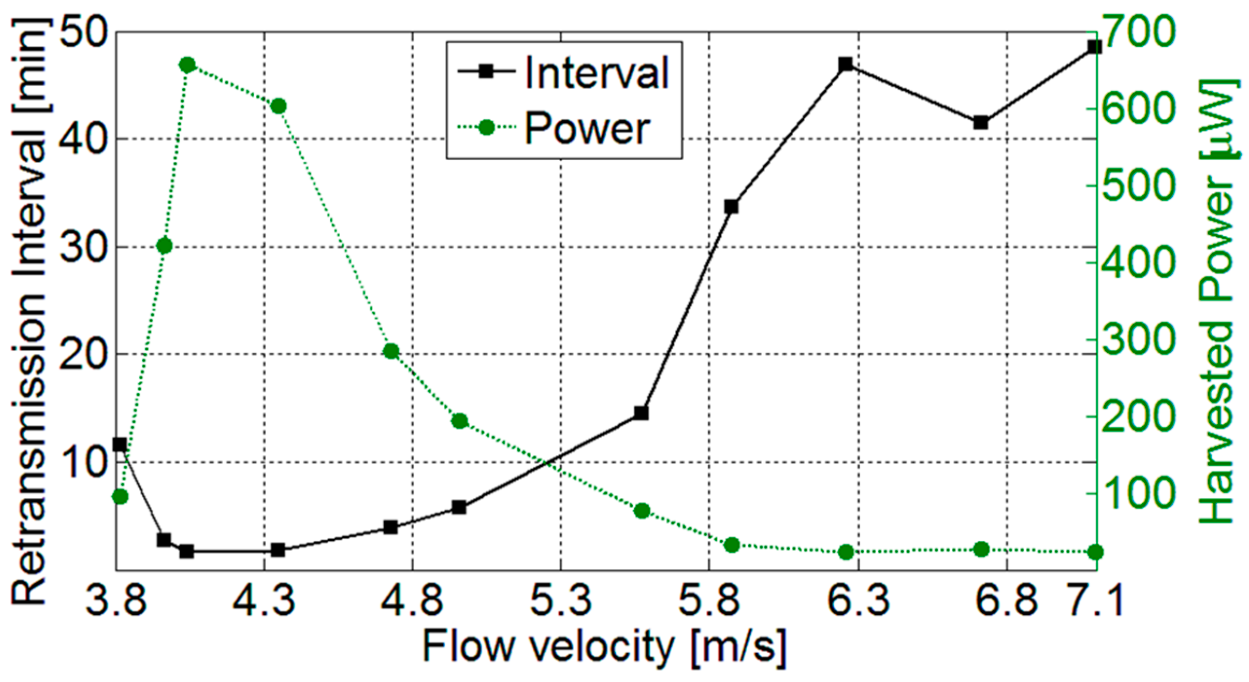
The measured power as a function of the flow velocity with the beam positioned at the orientation angle
θ = 300° is shown in
Figure 9. The power extracted from the system presents a cut-in velocity of the airflow of about 3 m/s. The largest power values, up to 1.3 mW, are obtained for intermediate velocities where the vortex repetition frequency is close to the beam resonant frequency. For higher velocities, the power tends to a constant value of about 0.2 mW. This trend to constancy can be ascribed to the combination of two opposite contributions occurring for increasing flow velocity and vortex repetition frequency in turn. There is a positive contribution due to the increasing magnitude of the forcing, and there is a negative contribution due to the decreasing response of the beam excited out of resonance by the increasing repetition frequency.
From the measured power on the optimal resistive load an estimation of the performances in terms of power density and conversion efficiency can be obtained for the proposed harvesting system. Considering the area of the piezoelectric converter plus the blade, a maximum power per unit area of about 40 μW/cm
2 is achieved. In addition, considering as the volume of the system the total region, comprising the bluff body, the beam with the converter, and the intermediate portion where the vortices arise, a maximum power density of about 2 μW/cm
3 can be calculated. The obtained power density and power per unit area are comparable to similar reported harvesting systems [
24,
26]. The conversion efficiency can be defined as the ratio of the output electrical power to the input available power associated to the airflow which hits the exposed surface of the bluff body. As stated by the Betz law, only a portion
cP ≈ 0.6 of the impinging power can be extracted from a mechanical-to-electrical converter. This portion goes down to
cP ≈ 0.3–0.4 for reduced dimensions of the converter, as in the case of the proposed system [
24]. Thus, the maximum electrical power as a function of the flow velocity can be calculated as:
where
S is the exposed surface of the bluff body and
ρair is the air density. The proposed system presents an efficiency
PL/Pel_max of up to about 1.7% for the flow velocity
u = 4 m/s where the maximum power is extracted.


