1. Introduction
Bathymetry is the measurement of underwater terrain, which is very important for a wide range of applications in hydrology, geomorphology, and meteorology. To date, several techniques for bathymetry retrieval have been developed for a variety of societal needs. The traditional bathymetry methods involve dropping a plumb line into the water or using a sonar system such as single-beam sonar, echo sounders, and multi-beam sounding [
1]. However, these methods are labor-consuming, time-costly, expensive, and are limited to the navigable area. In contrast, rapid and inexpensive remote sensing methods, including radar, hyperspectral imagery, and photogrammetry, have been developed to estimate bathymetry [
2]. These methods are better options than the in-situ measurement methods. However, radar and hyperspectral imagery cannot be used to directly retrieve water depth, and photogrammetry requires very clear water conditions [
3]. Meanwhile, their precision is relatively poor, and they cannot provide a high-resolution distribution (errors in the order of 1 m) [
4,
5,
6].
As an alternative, airborne light detection and ranging (LiDAR) bathymetry (ALB) has been developed as a powerful remote sensing technique that can be used to actively estimate bathymetry. By applying the ALB technique, the data can be obtained from waveform measurements of the received LiDAR pulse. This method can provide rapid operation with an acceptable accuracy and a high spatial density [
7,
8,
9,
10]. The ALB technique uses a pulsed blue-green laser as a bathymetric sensor that can penetrate the water to obtain the bathymetric data according to the differential arrival times of the laser echo signals reflected by the water surface and the sea bottom. In 1969, Hickman and Hogg first tested the performance of an airborne pulsed blue-green laser for near-shore bathymetric measurements [
11]. Subsequently, a lot of ALB systems were built and tested in different areas in the 1970s. An operational prototype ALB system named LARSEN-500 was developed in Canada in 1985. This system used a Q-switched dual-band laser, operating simultaneously at 532 nm and 1064 nm [
12]. Most of the early ALB systems were cumbersome to operate, and the costs were much higher than the other topographic systems. Moreover, a constant fraction discrimination (CFD) unit was used to retrieve the echo location by the airborne LiDAR scanner systems (ALSs), which only saves part of the time history of the returned LiDAR waveform.
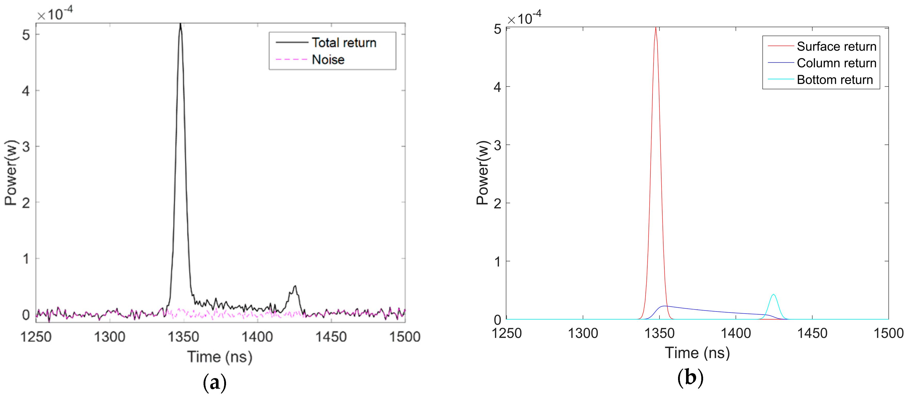
With the rapid development of LiDAR and computer technologies, ALB systems are becoming smaller, lower cost, and more powerful. To date (as of December 2016), the latest ALB systems such as CZMIL-Nova, RIEGL VQ-880-G, Leica Chiroptera-II, and HawkEye-III have been widely applied for shallow-water surveying [
13,
14]. All these ALB systems have small-footprint full-waveform digitizing capabilities, which has resulted in great progress in bathymetry accuracy and target resolution. In general, a typical sample of a bathymetric LiDAR waveform is composed of surface return, bottom return, volume backscattering, and background noise. The bathymetry estimates can be retrieved from the LiDAR waveform by the use of a waveform processing algorithm. To date, several LiDAR waveform processing algorithms have been developed for the processing of full-waveform airborne LiDAR. These algorithms can be grouped into three main classes: (1) echo detection [
15,
16,
17]; (2) mathematical approximation [
18,
19,
20,
21]; and (3) deconvolution methods [
22,
23,
24,
25,
26]. In order to compare the performances of these different methods, Wang et al. [
26] selected two algorithms for comparison in each class for single-wavelength bathymetric waveform processing, including peak detection (PD), the average square difference function (ASDF), Gaussian decomposition (GD), quadrilateral fitting (QF), Richardson-Lucy deconvolution (RLD), and Wiener filter deconvolution (WD). The results showed that the deconvolution methods excel in the accuracy of the water depth and the successful discovery rate, but their disadvantage is that they require the most time, due to the iterative step. The echo detection methods can obtain results in the shortest time, but their false discovery rate is higher than the other methods. The mathematical approximation methods require almost as much time as the deconvolution methods, and their accuracy is close to that of the echo detection methods. Based on continuous wavelet transform (CWT), Pan et al. [
27] presented a novel full-waveform processing algorithm which is more stable than the Gaussian or empirical system response decomposition methods for shallow-river bathymetry [
28]. From the comprehensive comparison of the different methods undertaken by Wang et al. [
26], it was found that the mathematical approximation methods are less cost-efficient than the other methods.
However, by using the mathematical approximation methods, the LiDAR bathymetric waveform can be fitted as a combination of mathematical functions. These mathematical functions can represent the surface return, bottom return, and the water column response. In particular, the water column contribution records the relationship between amplitude and time, and based on this relationship, we can estimate the diffuse attenuation coefficient (
Kd) and the chlorophyll concentration profile, and it is also possible to classify the ocean water type [
7,
29]. Therefore, it is important to develop suitable algorithms to fit the water column contribution in LiDAR waveforms, which can not only improve the accuracy of bathymetry retrieval, but also obtain the optical properties and ecological parameters of water [
30,
31]. To date, several mathematical approximation methods have been used to fit LiDAR bathymetry full waveforms. In Long et al. [
32], the water surface, water column, and water bottom contributions were approximated as a mixture of Gaussians. Abdallah et al. [
19] separately fitted the water surface, the water column, and the bottom contributions as a Gaussian function, a triangular function, and a Weibull function, respectively. Abady et al. [
20] developed a quadrilateral fitting algorithm, where two Gaussian functions were used to fit the surface and bottom contributions, and a quadrilateral function was used to fit the water column contribution. To sum up these mathematical approximation algorithms, it is relatively easy to fit the water surface and bottom returns, and the Gaussian function or Weibull function can show a satisfactory fit to the shape of the water surface or bottom contribution. However, the water column contribution is comparatively complicated, which is due to the fact that the water column contribution exhibits an asymmetric shape, physically corresponding to an infinite sum of successive translated Gaussian functions with an exponentially decaying amplitude along with water depth. Therefore, despite the fact that the above mathematical approximation algorithms are efficient, the fitting approaches cannot completely capture the physics of the interaction of the laser beam with the water column.
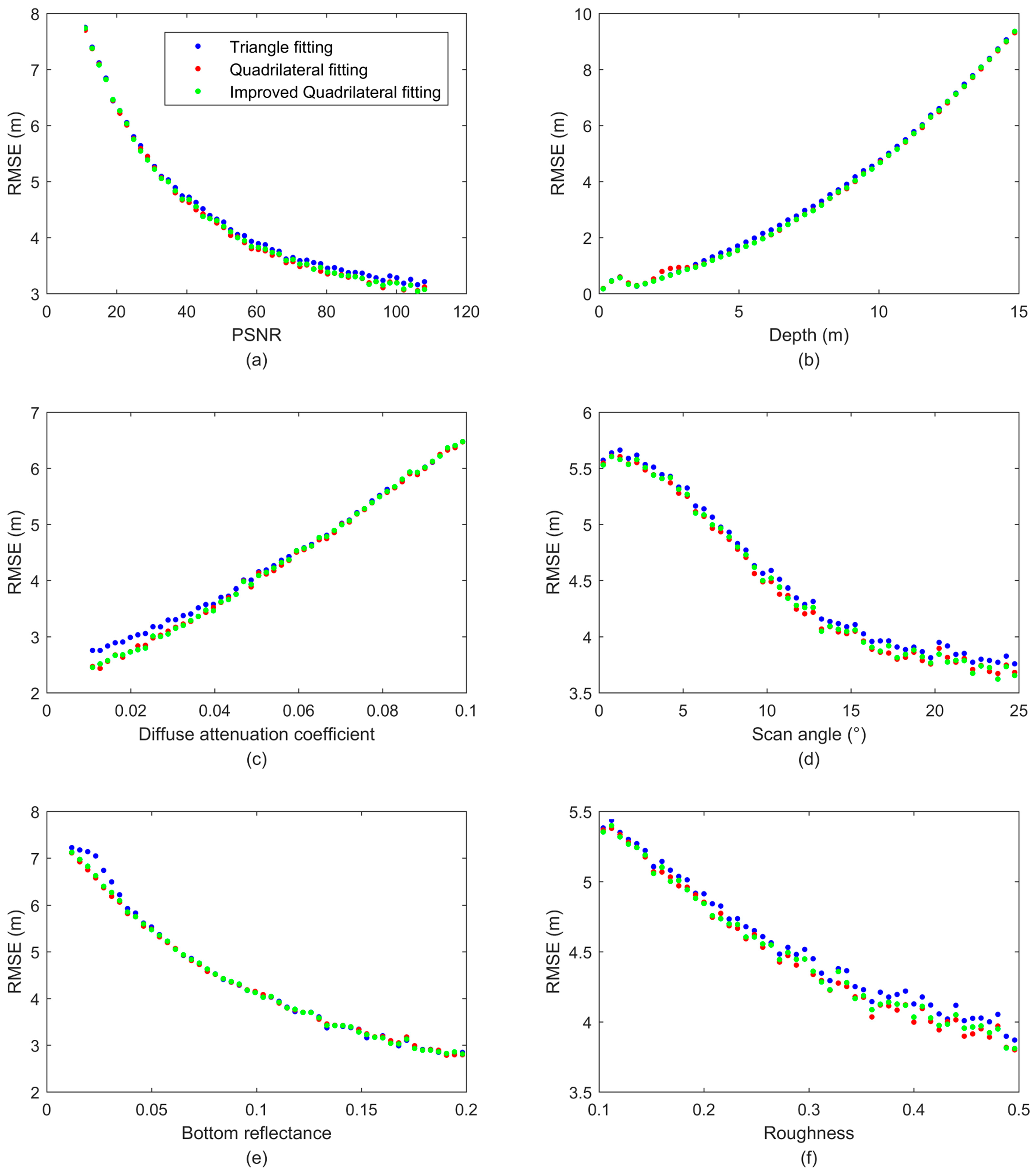
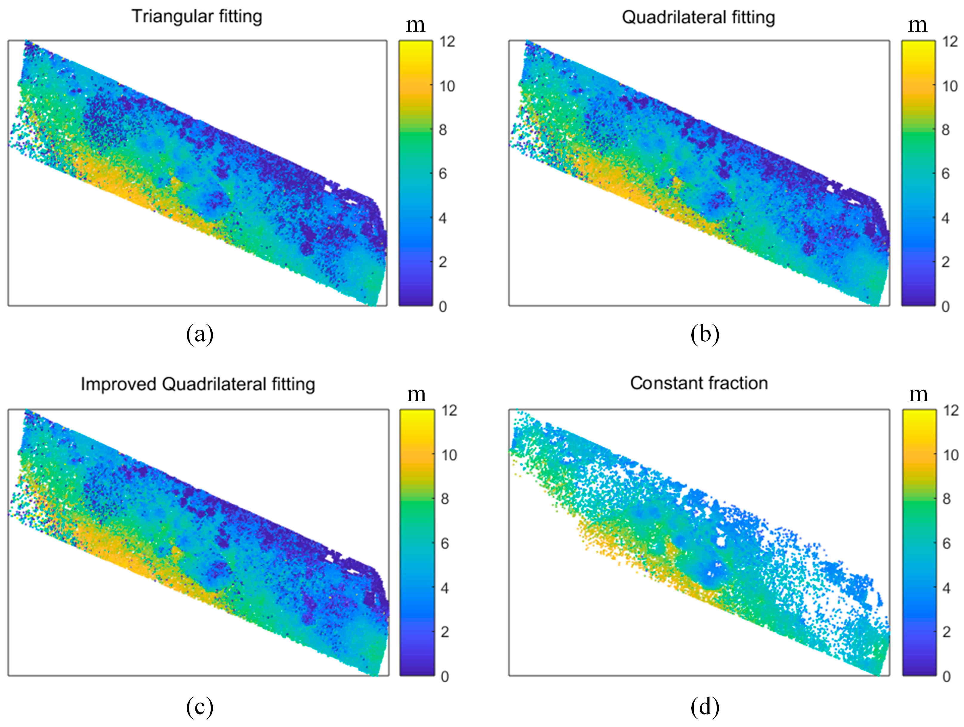
In this paper, we propose a new quadrilateral fitting algorithm to process bathymetric LiDAR waveforms and obtain bathymetry where: (1) Gaussian functions are used to fit both the surface and bottom components, and a new quadrilateral function is used to fit the water column contribution; (2) the new quadrilateral function is more in line with the fact that the water column response decreases exponentially with the increasing water depth; (3) the fittings are performed using a nonlinear least squares fitting approach according to the Levenberg-Marquardt algorithm [
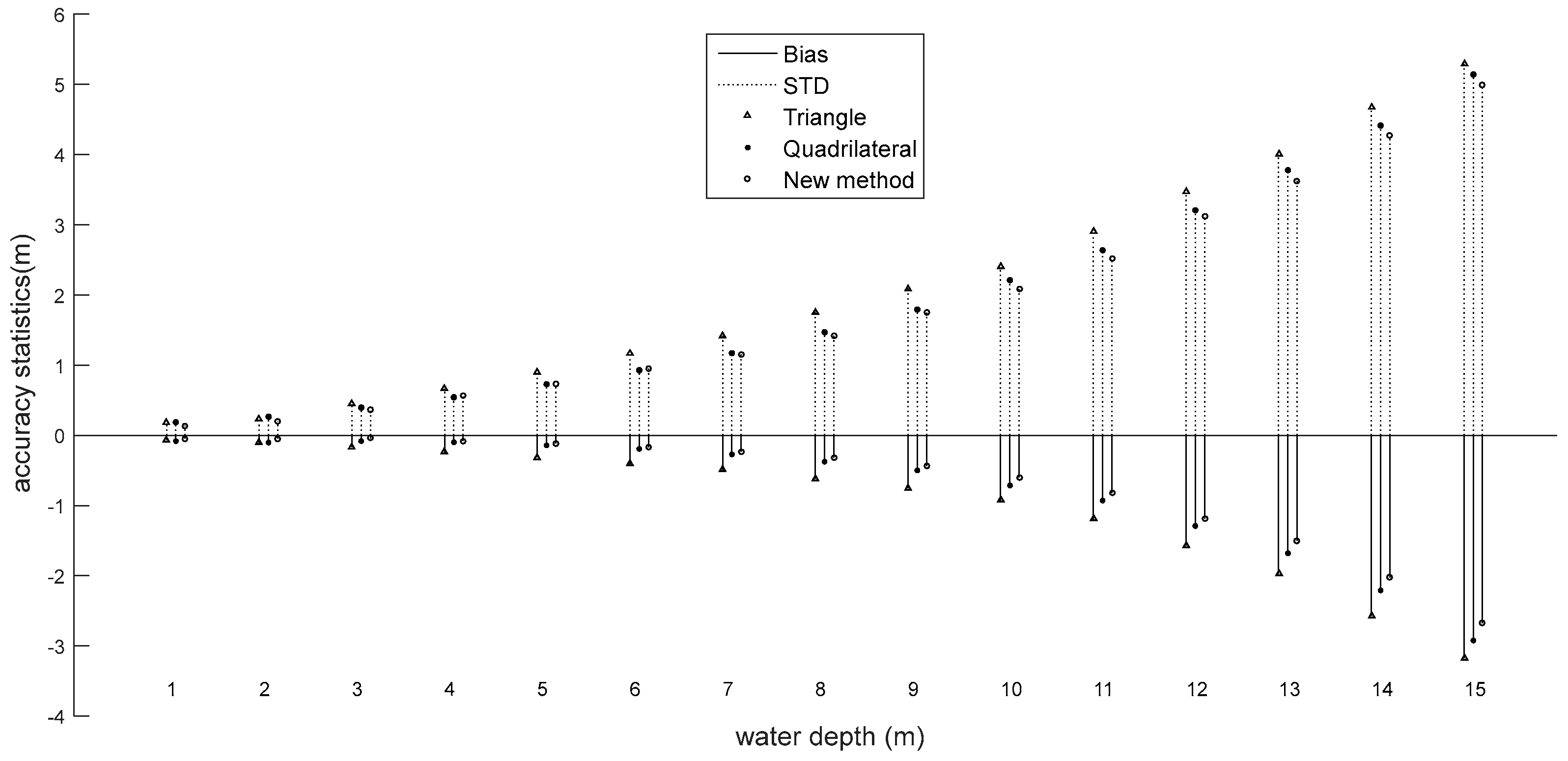
33]; and (4) we used a simulated dataset and a real dataset to test the presented waveform processing algorithm. The advantage of the new quadrilateral fitting algorithm we present was evaluated on sets of airborne simulated LiDAR waveforms and actual observed LiDAR waveform. In the following, for the simulated dataset, we compare the results of the bathymetry estimates (bias and standard deviation (STD)) obtained from the new quadrilateral function fitting method with those computed using a triangular function and the existing quadrilateral function initially presented by Abdallah et al. [
19] and Abady et al. [
19,
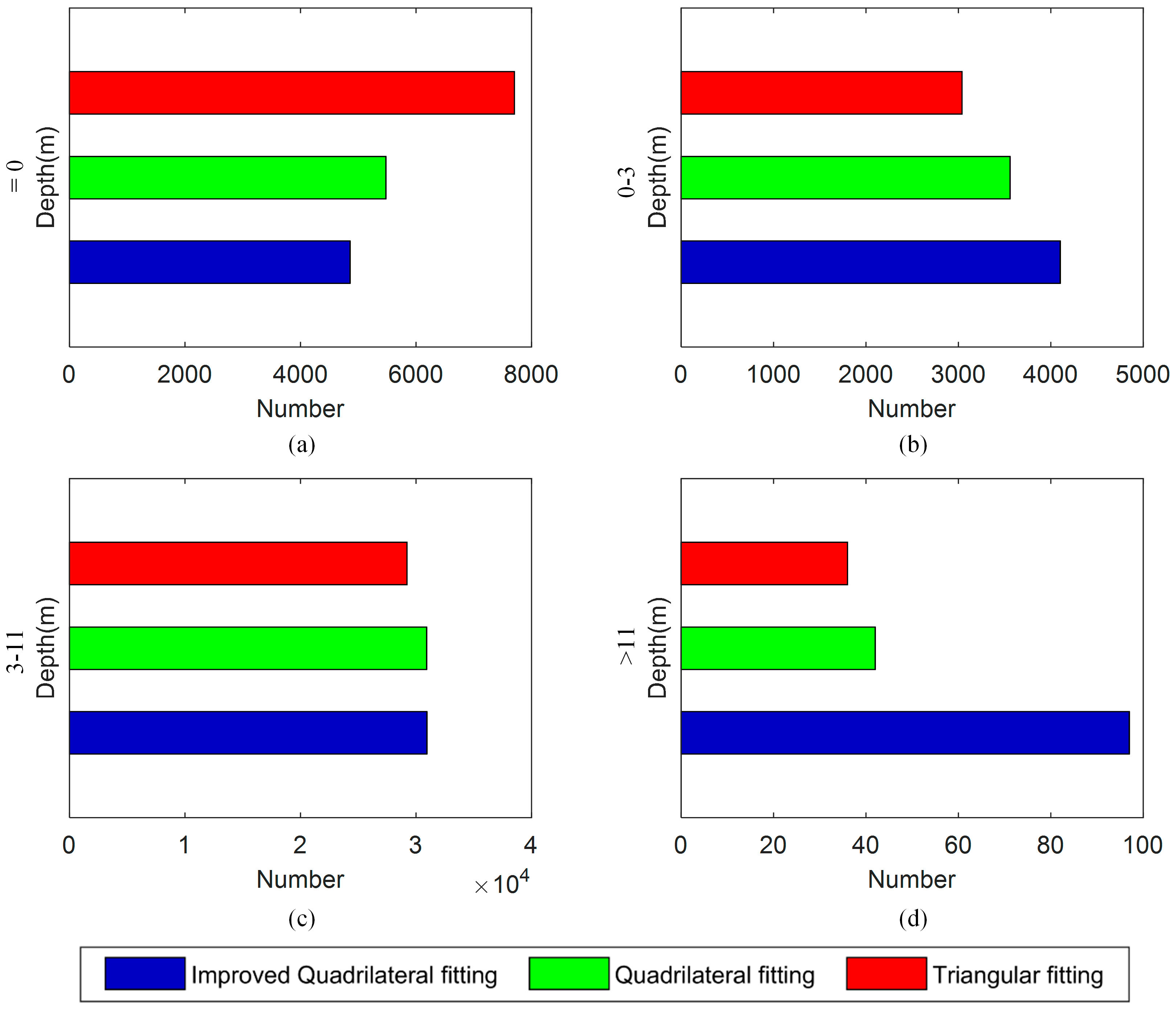
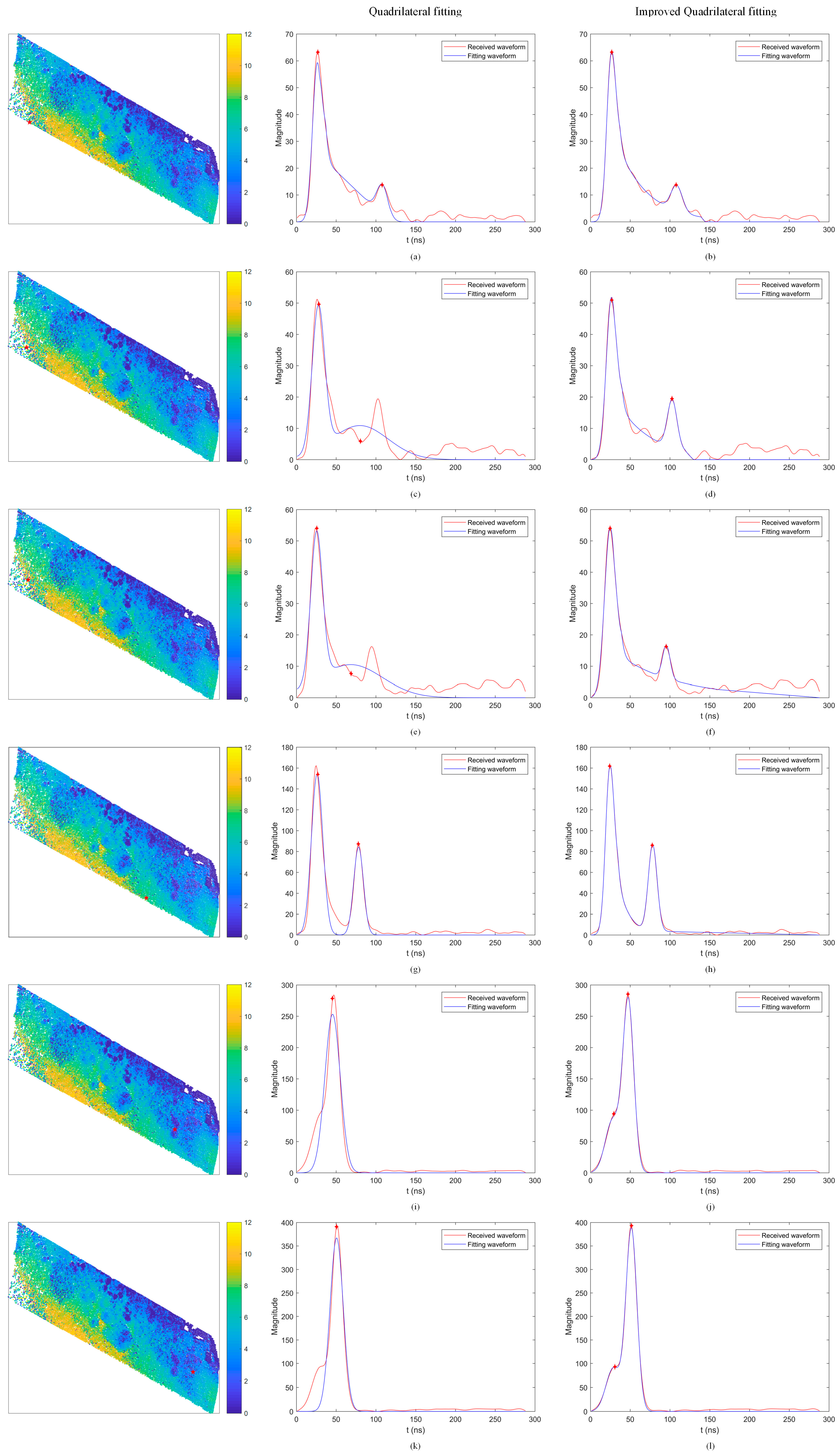
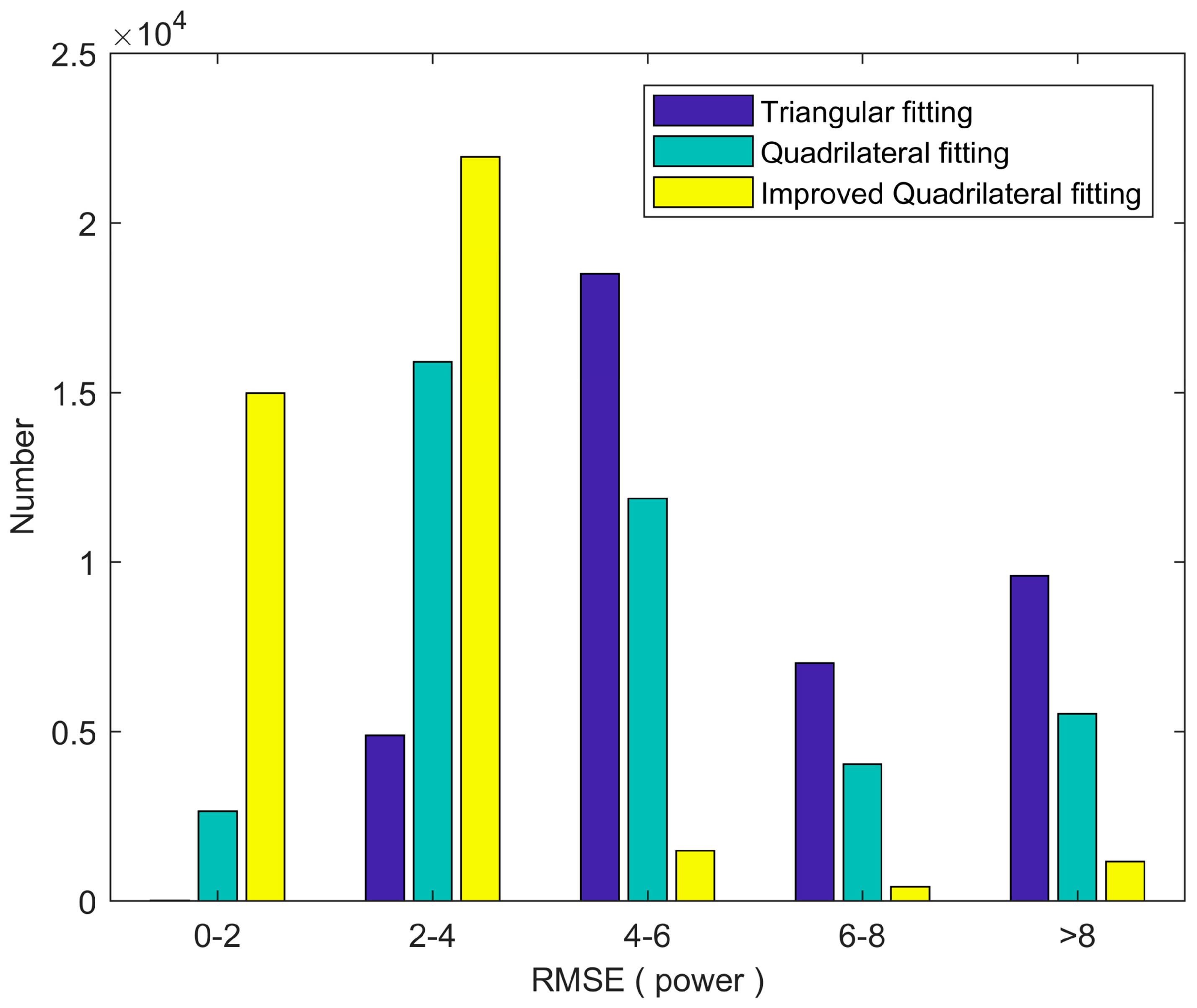
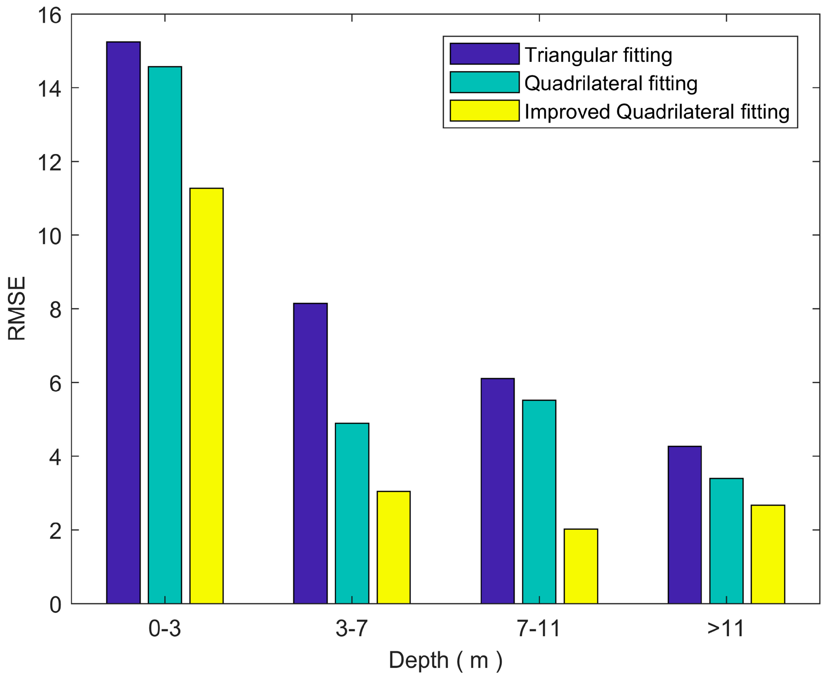
20], and we discuss the sources of bias and deviation. What’s more, we investigate the influence of the parameter settings on the accuracy of the bathymetry estimates. For the real dataset, we compare the number of points with two returns recognized and the noise from all the algorithms. In addition, we assess the fitting results of return waveforms and compute the root mean squared error (RMSE) between the fitting and true values of the amplitude of return waveforms by using different algorithms.

 ,
, 


