1. Introduction
Intersections are the meeting points of pedestrians, bicycles and vehicle flow, and junctions where road users change their directions. They are also the bottlenecks of urban roads, contributing a great deal to the loss of travel time due to traffic interference, management and control [
1]. Traditionally, intersection delay has been defined as the vehicle running time loss when turning or crossing intersections from upstream to downstream traffic flow [
2]. Based on floating car data, Wang further characterized travel time delay as a floating car’s travel time in excess of that of user-specified free flow travel time [
3]. The delay of intersections does not only affect the travel efficiency of road users but also the logic of signal control [
4]. It is estimated that delay at traffic signals contributes 5–10% of all traffic delay worldwide, exemplified by the statistics that 295 million vehicle-hours of delay occurred on major roadways in the USA each year [
5]. Thus, it is of striking importance for both real-time route planning and traffic control and management to accurately estimate time-dependent delay at intersections on urban road networks [
6].
In the existing traffic delay research, a wide range of traffic parameters has been explored, including the total travel time [
7], average waiting time [
8,
9], queue length [
10,
11,
12], throughput [
13], time delay [
14,
15], and number of stops [
16,
17]. The data sources mainly originated from simulation platforms or fixed road sensors (e.g., cameras and loops) [
18,
19,
20,
21]. Nevertheless, the traditional data have a number of intrinsic limitations [
22,
23], making it a challenge to the comprehensive evaluation of operation status at intersections based on the data.
The development of GPS (Global Position System) technologies enables us to utilize floating cars (i.e., vehicles equipped with GPS devices) to track vehicle trajectories and collect real-time traffic data across the entire road networks. The vehicles can be regarded as ubiquitous mobile sensors, probing a city’s rhythm and pulse with high data collection efficiency [
24,
25,
26]. Compared with the conventional data sources, the floating car data (FCD) provide three important advantages. First, real-time traffic data can be collected, and automatically sent to a processing center where information about traffic conditions is extracted [
27]. Secondly, the intersections of a large part of the road network can be monitored, having a much larger coverage than sensor data by which only a limited number of areas can be observed [
28]. Thirdly, via GPS-equipped vehicles, high-quality data are collected with low costs [
29]. All these characteristics have led to FCD gradually becoming the mainstream data collection method in transportation research [
30].
Studies have been conducted to extract traffic parameters from the FCD data, based on map-matching and Geographic Information System (GIS) techniques [
31,
32]. However, there are two major obstacles in applying these techniques to the analyses of intersections. First, it has been generally acknowledged that map-matching is a complicated and time consuming tool [
33], making it challenging to match massive amounts of FCD across whole urban intersections [
34]. Secondly, it is difficult to acquire a high quality and timely updated map which ensures the accuracy of the matches. Thus, despite the fact that FCD provide important information about traffic patterns of urban road networks [
35], there has been a lack of methodologies which focus on the comprehensive evaluation of operation status at intersections using the data. To fill in this gap, in this study, a novel traffic grid model has been proposed, which is based on the FCD data but assesses the operational status at intersections more efficiently. The aim is to provide accurate estimation of traffic operation states at intersections across the whole urban road networks, and evaluate and diagnose serious problems (e.g., time delay) at the intersections. The final goal is to assist traffic managers in designing optimal measures to increase traffic operation efficiency and reduce traffic delay at urban intersections.
Compared to the existing literature, the proposed method has the following major advantages. (1) It is completely based on the data, without the aid of any additional tools such as complex map-matching and digital maps. This makes this approach particularly practical for researchers and engineers who are not familiar with the map-matching and GIS techniques. (2) This method is easily transferred to other cities for the evaluation of traffic operation at most of the signalized intersections of the urban road networks. (3) Under the grid modelling, the intersections are transformed into discrete cells, and the FCD data are matched to the grids through a simple assignment process. (4) From the constructed cell-based intersections, key traffic parameters are extracted, and intersections with the longest delay are identified and the detailed problems at these intersections are further diagnosed. The simplicity of the grid model and the parameter extraction, along with the constant input of the GPS data, makes the proposed method highly efficient in evaluating and diagnosing intersection operation in real time.
Using the central area of Beijing as the case study, the potential and feasibility of the proposed method are demonstrated. The rest of this paper is organized as follows.
Section 2 describes the FCD data and details the proposed methodology.
Section 3 conducts a case study and in-depth analyses on the experimental results. Finally,
Section 4 ends this paper with major conclusions and discussions for future research.
3. The Empirical Case Study in Beijing
The data used in this case study include 2,712,744 floating cars’ trajectories (i.e., 35.7 GB in size) collected from 1 to 15 in August 2017, in the central area of Beijing with longitudes and latitudes as follows: <116.399450, 116.431700> and <39.947934, 39.966344>. In the study area, eight intersections were selected, namely, NO.1–NO.8 (See
Figure 5), and they cover various types of intersections, including the intersecting of both arterial and branch roads (i.e., NO.2, NO.3, NO.6, NO.7, NO.8), only arterial roads (i.e., NO.4 and NO.5), and only branch roads (i.e., NO.1).
Figure 6 shows the distributions of the averages of hourly and daily traffic flows across all the selected intersections. It was noted that the traffic flow in the evening peak hour (i.e., 17:00–19:00) was larger than in other periods, including the morning rush hour (i.e., 7:00–10:00) and the off-peak period (e.g., 14:00–16:00) (See
Figure 6a); while during the week, the flow was larger on workdays than on non-workdays (See
Figure 6b).
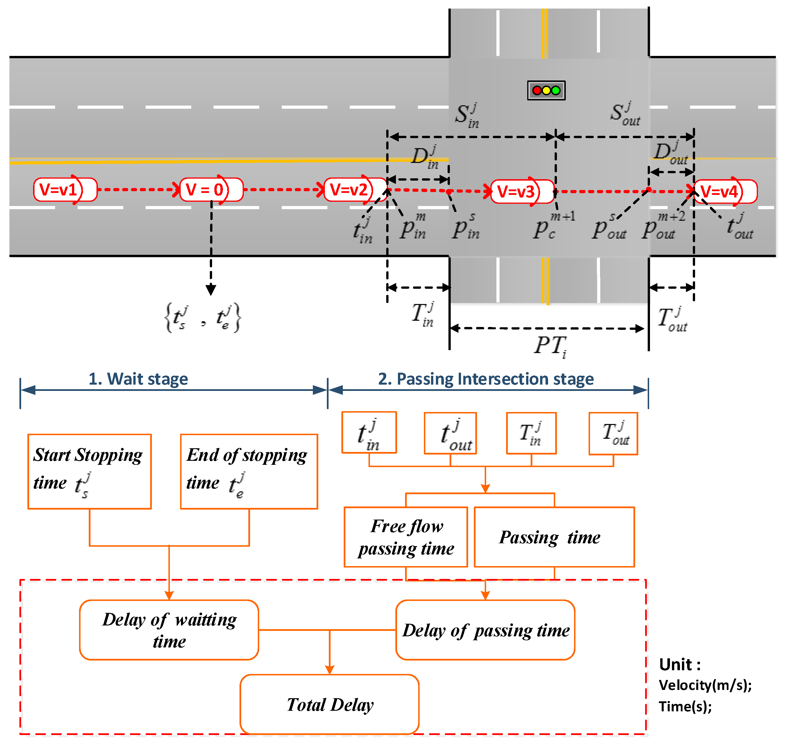
3.1. The Intersections’ Total Delay
To analyze the total delay at each of the intersections, we construct the spatial-temporal diagrams with the time slices of 30 min (
Figure 7a), 15 min (
Figure 7b) and 5 min (
Figure 7c), respectively. For each intersection (indicated by the y-axis), the different levels of delay along the different times of the day (indicated by the x-axis) are described using a color scheme, with the darkest blue referring to the shortest delay (i.e., Level A) and the darkest red to the longest one (i.e., Level F). Moreover, all eight intersections are sorted in terms of their total delay, and this order is indicated with the arrow on the left side of these figures. It was observed that the delay at the NO.2 intersection was the longest, particularly during the morning and evening rush hours. However, the delay at the NO.7 intersection was the shortest, which could be due to the fact that it is forbidden to make a left turn at this intersection.
Figure 8 further details of the distribution of the delay with the slice of 5 min during the two peak periods. It shows that the delay at intersection NO.2 reached the longest at 8:00–9:30 in the morning, and at 17:00–19:45 in the evening.
3.2. The Traffic Operation States for Individual Intersections
Apart from the total delay, other major traffic parameters including the traffic flow, average velocity and delay in each direction of each of the intersections are further investigated. In the following, the intersection with the longest delay among these selected ones, i.e., NO.2. intersection, is analyzed. The same process can be applied to any of the remaining intersections.
3.2.1. The Traffic Delay
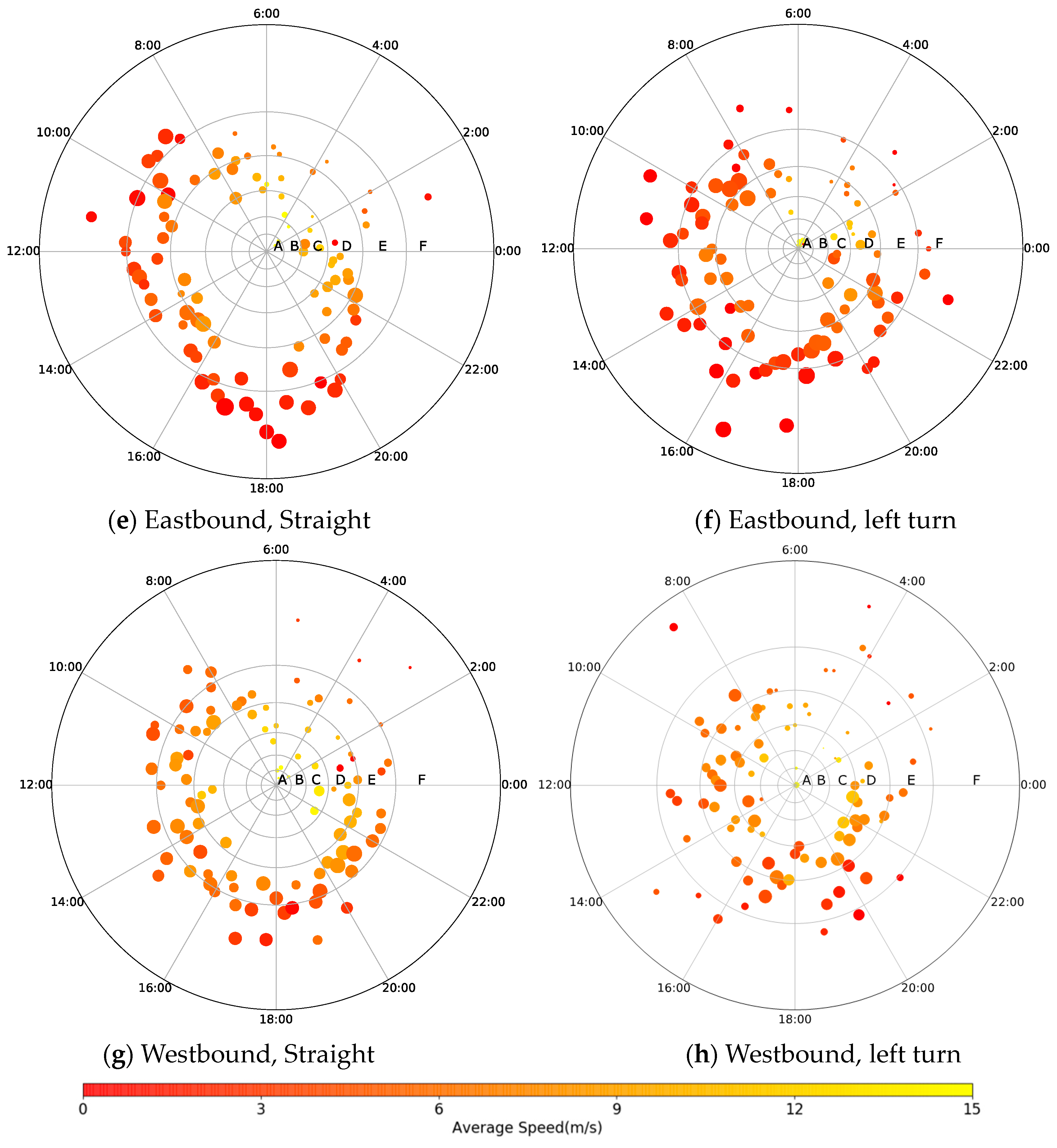
Figure 9 describes the distribution of these three major parameters across different times of working days at the intersection, using the time slice of 15 min. Each point depicts a vector of three values of these parameters, including the traffic volume (i.e., represented by the size of the point), the average velocity (m/s) (i.e., represented by the color of the point), and the delay level (i.e., represented by the radius of the point at the polar coordinates). A point that is further from the origin of the coordinates and has a larger size and red color refers to a traffic state featured with more traffic volume, lower speeds, and longer delay.
From
Figure 9, it was noted that the traffic flows in the south- and northbound straight directions (See
Figure 9a,c) were higher than those of the east- and westbound straight directions (See
Figure 9e,g). When the conditions between the south- and northbound directions were compared, the northbound traffic flow was lower, its traffic speed was slower, and therefore the corresponding traffic delay was shorter.
From
Figure 9b,d, it was found that the distributions of the traffic flow and average velocity for the southbound and northbound left turn directions are similar. However, the southbound left turn had the longest delay during 16:00–20:00, while the northbound left turn suffered the worst delay problem at 10:00–14:00.
Figure 9e–h further show that the eastbound traffic average speeds for both the straight and left turn directions were much slower than the westbound average speed. Consequently, the delays in the eastbound directions were longer, particularly during the morning and evening rush hours.
In summary,
Table 4 lists all of the key traffic performance parameters of the eight critical directions for the intersection.
3.2.2. The Traffic Speed
For further analysis of the average speed, we compared the distribution of the average speed among different directions of the intersection, as depicted in
Figure 10. A clear distinction was observed in the speeds between the straight and left turn directions in each of the southern or northern routes (See
Figure 10a). In contrast, there was no large difference between the speeds of the straight and left turn directions for each of the eastern or western routes (See
Figure 10b). This suggests that there would be a protected left-turn phase for the south- and northbound flows, causing little interference to the go-straight traffic. However, there was no protected left-turn designed for the east- and westbound flows.
3.2.3. The Ratio of Non-Stop FCD to Stop FCD
Figure 11a shows the total number of stop trajectories over the entire day across different directions of the intersection, indicating that the numbers in the south- and northbound straight directions (i.e., 33% and 31%, respectively) were much higher than those in the east- and westbound straight directions (i.e., 3% and 2%, respectively). On the contrary, the numbers of stop trajectories in the left turn of all the north-, south-, east- and westbound directions were similar (i.e., 3.2%, 2.6%, 3.0% and 1.7%, respectively). However, according to the ratio (
) between the number of non-stop trajectories and that of stop ones, as described in
Figure 11b,
was much lower in the left turn of the north- and southbound directions (i.e., 10.11% and 16.18%, respectively) than that of the east- and westbound directions (i.e., 66.08% and 76.18%, respectively). This indicates that the number of non-stop trajectories was smaller and the traffic conditions were worse in the left turn of the north- and southbound directions than in the east- and westbound directions.
Figure 11c,d further depict the values of
during the morning and evening rush hours, respectively. It was observed that
in the left turn of the north- and southbound directions in these two periods (i.e., 7.25% and 7.48% in the morning and 8.76% and 7.31% in the evening) was lower than that for the entire days (i.e., 10.11% and 16.18% as shown in
Figure 11b). This suggests that in the peak period, the unreasonable timing of signal lights would be unable to match the increasing of traffic flow. Moreover,
in the northbound straight direction during the morning peak (i.e., 68%) was lower than that in the evening peak (i.e., 115%). Meanwhile, an opposite trend was observed in the southbound straight direction, in which
is higher in the morning (i.e., 104%) and lower in the evening (i.e., 90%). This indicates the existence of a tidal phenomenon in the traffic flow between the north- and southbound straight directions.
In summary,
Table 5 lists all of the number of stops and the ratio of the number of non-stop cars to the number of stop ones of the eight critical directions for the intersection.
3.3. Diagnosis of the Delay Problems for Individual Intersections
Figure 12 characterizes the distribution of
(i.e., the ratio between the flow ratio and the green time ratio) over different directions of the intersection in each of the phases. It should be noted that
values of the north- and southbound straight directions were greater than those in other directions.
Table 6 further lists the specific parameter values of
and
in each phase of each time scheme. It indicates that the minimum
values in north- and southbound straight directions phase were greater than that in the other phases in all the timing schemes. This implies that the effective green time of phase of the north- and southbound straight direction would be much shorter than it should be, which leads to the longer delay in the corresponding directions of the intersection.
4. Discussion and Conclusions
In this study, a novel traffic grid algorithm was proposed, which is based on the FCD data but makes the map-matching process for signalized intersections more efficient. Furthermore, it provided an accurate estimation of traffic operation states at the intersections and an efficient traffic performance evaluation for signalized intersections at the network level, and can be applied to diagnose the specific problems for individual intersections.
The traditional data-collecting devices cover only fixed points of the traffic network, such as loop detectors, which are impossible to produce reliable information about travel time within the network [
45]. In comparison, based on the massive amount of FCD data that are highly spatial-temporal detailed, their 3s sampling rate guarantees the accurate estimation of these intersections’ operation parameters. This study selected three kinds of time dimensions (i.e., 5 min, 15 min, 30 min) as the time slices to describe the intersections’ operation states. As for the traffic analysis region of defined intersection, Zhang et al. defined a fixed one with a 200 m length from the center of an intersection to a 100 m distance from upstream and downstream directions [
41]. The fixed analysis region may cause an inaccurate estimation of the traffic parameters because the upstream queue lengths might be frequently beyond the 100 m limit, especially for large-scale intersections. In this study, the differences of intersections’ configurations and the spatial-temporal FCD’ distributions were considered, and the region sizes are variable corresponding to the actual traffic performance, which guaranteed the assurance of the veracity of the arithmetic.
In previous studies, only one or two traffic parameters (e.g., delay and stop rate) were used for intersection performance analyses, which were insufficient to explore the traffic operation performance deeply [
46]. Using the radar figures (e.g.,
Figure 9), we combined the three traffic parameters (i.e., time delay, traffic flow, average speed) to estimate the traffic intersection operation state and evaluate the intersections’ levels of service. Thus, the intersections’ operation performances in the network can be sorted, and the ones with the worst performance can be identified. The intersections with the serious delay problems can be further investigated in terms of the traffic condition in different directions. It was found that there was a significant difference in the average speed between the straight and the left turn directions when unprotected left-turn phases were applied, which is consistent with the studies of Angell et al. and Wang et al. [
47,
48]. In addition, the ratio of non-stop to stop FCD (
) also exhibits variations across different times of the day and in different directions. Particularly, a tidal phenomenon of traffic flow during the morning and evening peak hours was discovered. Traffic engineers should take the tidal phenomenon into consideration when designing traffic signal control strategies. For the individual intersections, the traffic delay problem can be further diagnosed based on the parameter
. The value of the parameter is either larger or smaller than one, indicating imbalanced signal phasing design issues for the intersections, which can be utilized as an efficient tool for individual intersections’ signal phase readjustment.
Owing to unavailability of loop detector data for the case study, we could not examine the floating cars’ penetration ratio in the total traffic. However, this study focuses on the traffic signal intersection performance evaluation. The huge numbers of FCD can sufficiently reflect the historical traffic conditions and accurately provide travel speed information. Therefore, the comparative results of levels of service between the intersections in the traffic networks and the diagnoses of signal phasing design issues for individual intersections should be reliable. In future work, if the loop detector data are available, it is suggested to consider the floating cars’ penetration ratio in total traffic in order to provide more detailed methods for the real-time cases that the samples of FCD are insufficient during some cycles.


