Robust Least-SquareLocalization Based on Relative Angular Matrix in Wireless Sensor Networks


Abstract
1. Introduction
1.1. Related Works
1.2. Contributions
- A sufficient and unnecessary condition for the LS cost function to be convex is proposed and proven for WSN positioning.
- We define the relative angle matrix for both noncooperative and cooperative scenarios and show that the LS function can be transformed into a globally convex function if all the targets are located inside the convex polygon formed by its adjacent nodes.
- A robust algorithm that detects the relative angular matrix is proposed for WSN localization. Additionally, we improve the algorithm by using angle constraints so that it can be used in both the AOA/TOA and TOA positioning methods, which extends the applicability of the method.
2. Definition and Scenario Description
2.1. Definition of the Nodes and Links
2.2. Definition of the Errors
2.3. Noncooperative Scenario Description
2.4. Cooperative Scenario Description
3. Convex Analysis of the Model
3.1. Analysis of the Noncooperative Scenario
3.2. Analysis of the Cooperative Scenario
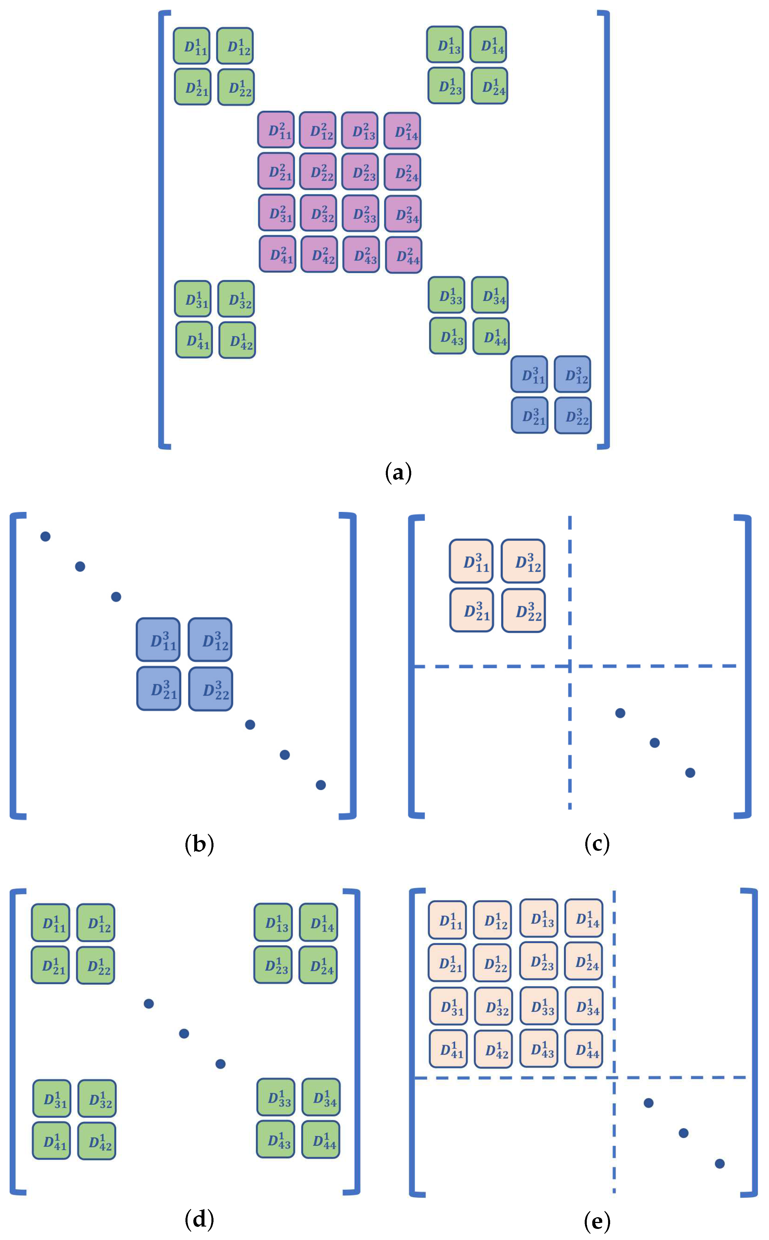
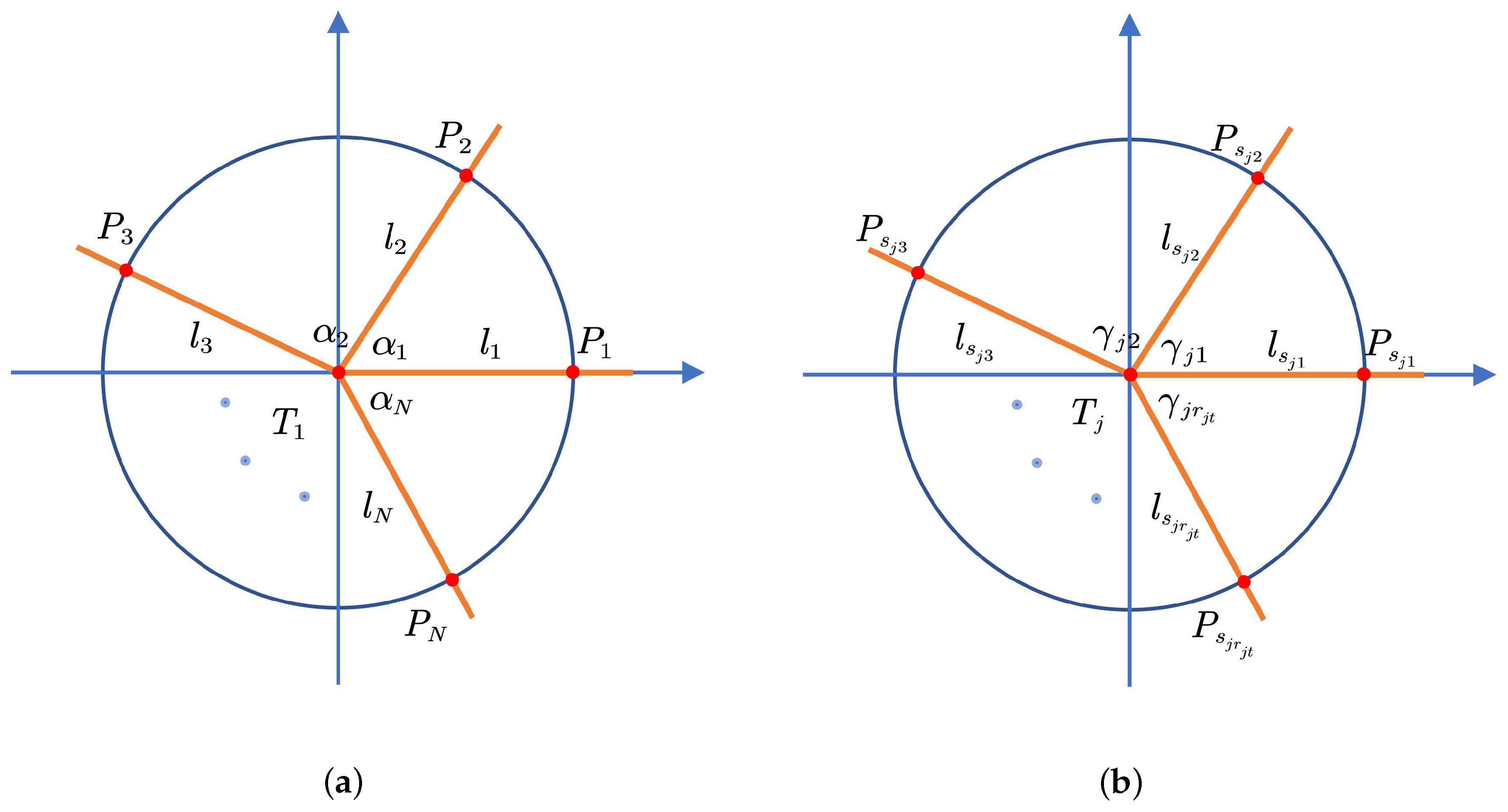
4. Null Space of the Relative Angle Matrix
4.1. Definition of the Relative Angle Matrix
4.2. Null Space Algorithms
- How do we achieve ?
- For an arbitrary , does satisfy the condition of ?
- When there are errors in , how do we deal with them?
| Algorithm 1: A-NLS and C-NLS algorithms. |
| Input: and (the angle observation is unnecessary for C-NLS); |
| Output: |
| 1: Measuring or calculating that entails errors; |
| 2: Angle estimation is performed by using the Equation (45); |
| 3: Obtain ; |
| 4: Calculate the null space of , and choose the appropriate so that ; |
| 5: For , calculate , set , , and choose random ; |
| 6: while do |
| 7: Update for using the Gauss–Newton iteration method; |
| 8: ; |
| 9: end while |
| 10: return |
5. Simulations and Results
5.1. Simulation Scenario Setting
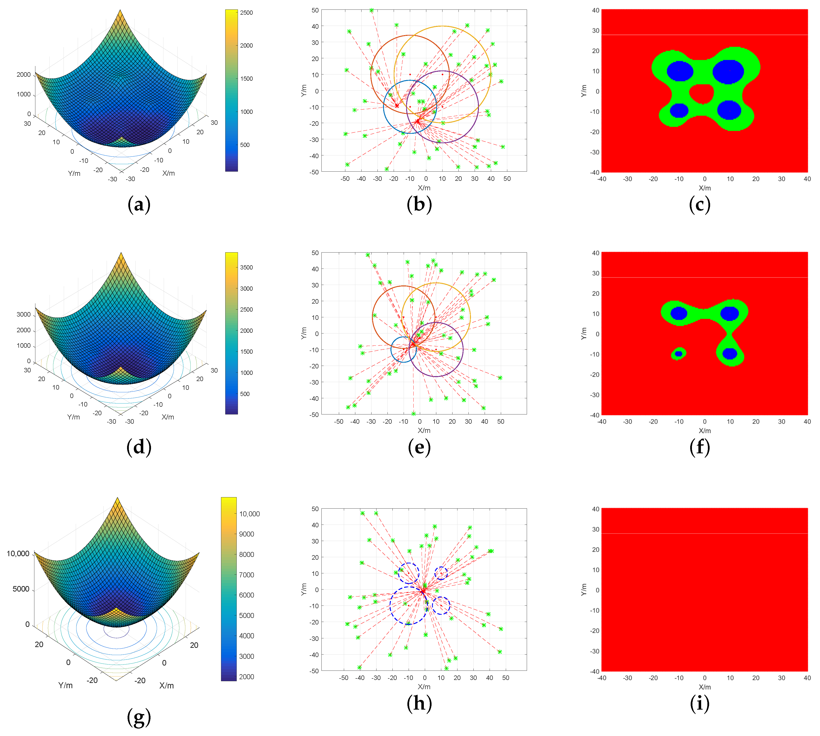
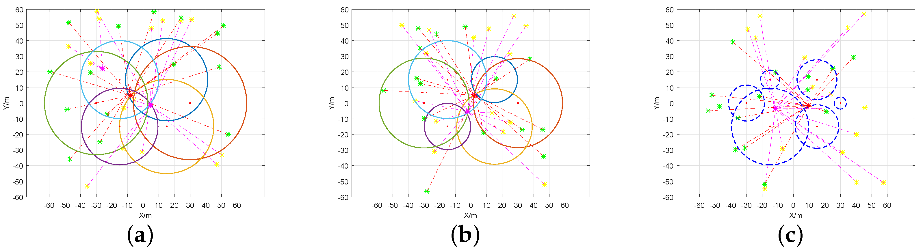
5.2. Convexity Verification
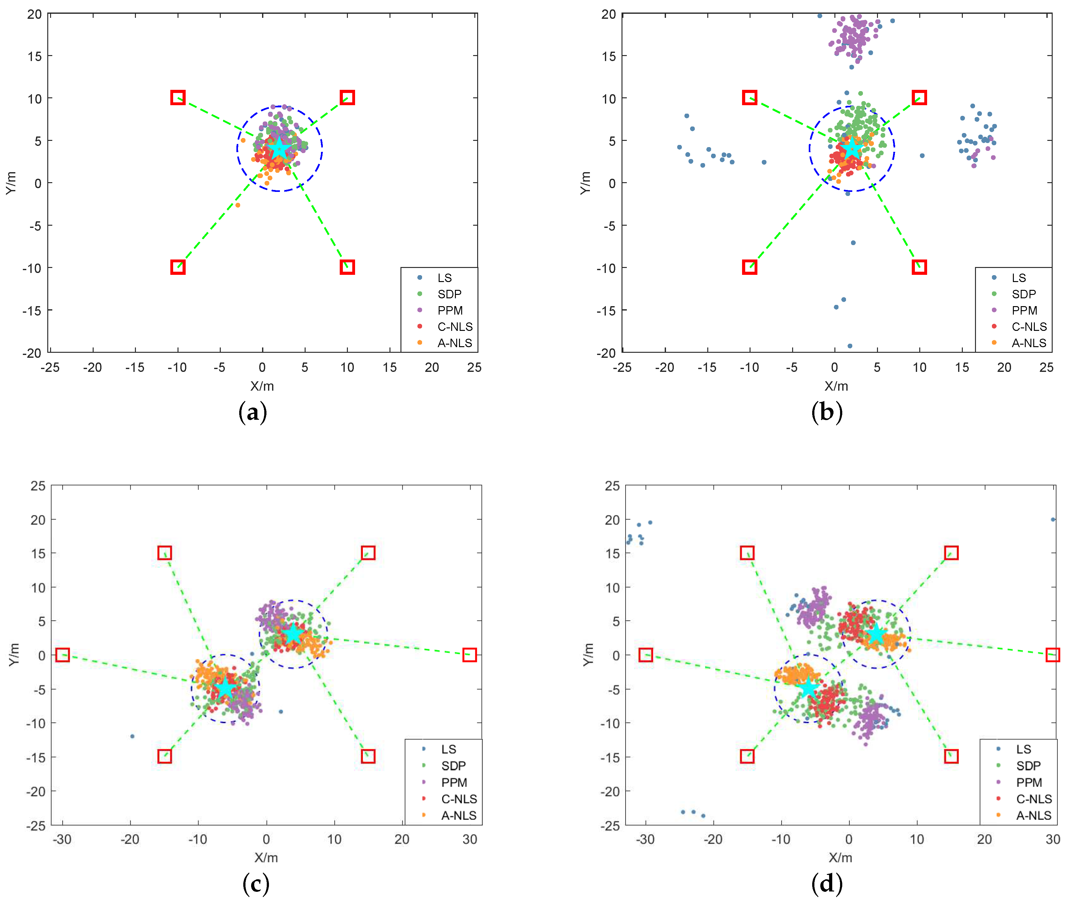
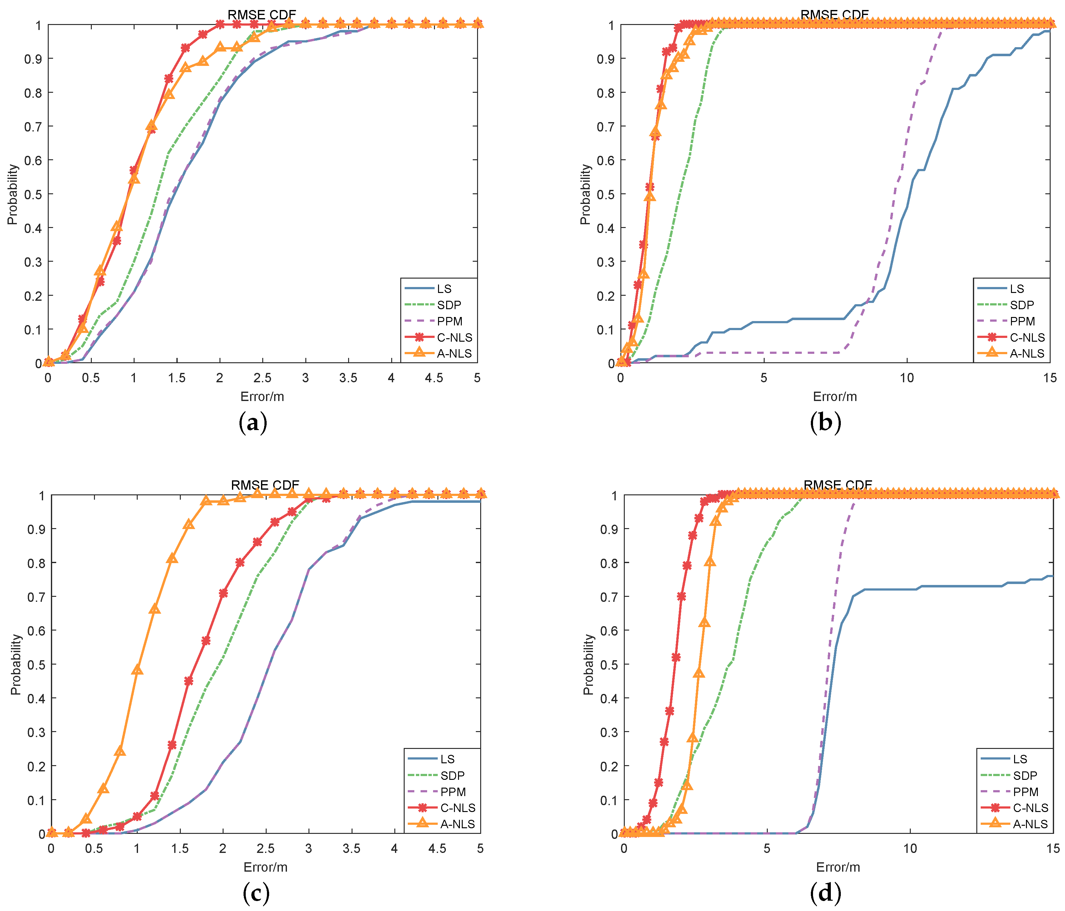
5.3. Null Space Algorithm Performance
6. Conclusions
Author Contributions
Funding
Conflicts of Interest
Appendix A
Appendix B
Appendix C

References
- Tian, S.; Dai, W.; Li, G.; Lv, J.; Xu, R.; Cheng, J. On the Research of Cooperative Positioning: A Review. In Proceedings of the 4th China Satellite Navigation Conference, Wuhan, China, 15–17 May 2013. [Google Scholar]
- Parkinson, B.W. Global Positioning System: Theory and Applications, Volume II; American Institute of Aeronautics and Astronautics (AIAA): Reston, VA, USA, 1996; Volume 163. [Google Scholar]
- Witrisal, K.; Meissner, P.; Leitinger, E.; Shen, Y.; Gustafson, C.; Tufvesson, F.; Haneda, K.; Dardari, D.; Molisch, A.F.; Conti, A. High-Accuracy Localization for Assisted Living: 5G systems will turn multipath channels from foe to friend. IEEE Signal Process. Mag. 2016, 33, 59–70. [Google Scholar] [CrossRef]
- Shahmansoori, A.; Garcia, G.E.; Destino, G.; Seco-Granados, G.; Wymeersch, H. Position and Orientation Estimation Through Millimeter-Wave MIMO in 5G Systems. IEEE Trans. Wirel. Commun. 2018, 17, 1822–1835. [Google Scholar] [CrossRef]
- Jiang, L.; Cai, B.G.; Jian, W. Cooperative Localization of Connected Vehicles: Integrating GNSS with DSRC Using a Robust Cubature Kalman Filter. IEEE Trans. Intell. Transp. Syst. 2017, 18, 2111–2125. [Google Scholar]
- Shen, Y.; Win, M.Z. Fundamental Limits of Wideband Localization and mdash; Part I: A General Framework. IEEE Trans. Inf. Theory 2010, 56, 4956–4980. [Google Scholar] [CrossRef]
- Shen, Y.; Wymeersch, H.; Win, M.Z. Fundamental Limits of Wideband Localization—Part II: Cooperative Networks. IEEE Trans. Inf. Theory 2010, 56, 4981–5000. [Google Scholar] [CrossRef]
- Penna, F.; Caceres, M.A.; Wymeersch, H. Cramer-Rao Bound for Hybrid GNSS-Terrestrial Cooperative Positioning. IEEE Commun. Lett. 2010, 14, 1005–1007. [Google Scholar] [CrossRef]
- Gante, A.D.; Siller, M. A Survey of Hybrid Schemes for Location Estimation in Wireless Sensor Networks. Procedia Technol. 2013, 7, 377–383. [Google Scholar] [CrossRef][Green Version]
- Buehrer, R.M.; Jia, T. Collaborative Position Location; Wiley-IEEE Press: New York, NY, USA, 2011; pp. 1089–1114. [Google Scholar]
- Xiong, Z.; Sottile, F.; Caceres, M.A.; Spirito, M.A.; Garello, R. Hybrid WSN-RFID cooperative positioning based on extended kalman filter. In Proceedings of the 2011 IEEE-APS Topical Conference on Antennas and Propagation in Wireless Communications, Torino, Italy, 12–16 September 2011. [Google Scholar]
- Sottile, F.; Wymeersch, H.; Caceres, M.A.; Spirito, M.A. Hybrid GNSS-Terrestrial Cooperative Positioning Based on Particle Filter. In Proceedings of the 2011 IEEE Global Telecommunications Conference, Kathmandu, Nepal, 5–9 December 2011. [Google Scholar]
- Chen, L.; Wen, F. Received Signal Strength based Robust Cooperative Localization with Dynamic Path Loss Model. IEEE Sens. J. 2016, 16, 1265–1270. [Google Scholar]
- Bao, D.; Hao, Z.; Hao, C.; Liu, S.; Zhang, Y.; Feng, Z. TOA Based Localization under NLOS in Cognitive Radio Network; Springer Press: New York, NY, USA, 2016; pp. 668–679. [Google Scholar]
- Tomic, S.; Beko, M.; Rui, D.; Montezuma, P. A Robust Bisection-based Estimator for TOA-based Target Localization in NLOS Environments. IEEE Commun. Lett. 2017, 21, 2488–2491. [Google Scholar] [CrossRef]
- Nguyen, T.L.N.; Vy, T.D.; Shin, Y. An Efficient Hybrid RSS-AoA Localization for 3D Wireless Sensor Networks. Sensors 2019, 19, 2021. [Google Scholar] [CrossRef]
- Ji, L.; Conan, J.; Pierre, S. Mobile Terminal Location for MIMO Communication Systems. IEEE Trans. Antennas Propag. 2007, 55, 2417–2420. [Google Scholar]
- Goulianos, A.A.; Freire, A.L.; Barratt, T.; Mellios, E.; Beach, M. Measurements and Characterisation of Surface Scattering at 60 GHz. In Proceedings of the 2017 IEEE 86th Vehicular Technology Conference (VTC-Fall), Toronto, ON, Canada, 24–27 September 2017. [Google Scholar]
- Vaghefi, R.M.; Buehrer, R.M.; Wymeersch, H. Collaborative Sensor Network Localization: Algorithms and Practical Issues. Proc. IEEE 2018, 106, 1089–1114. [Google Scholar]
- Shang, Y.; Rumi, W.; Zhang, Y.; Fromherz, M. Localization from Connectivity in Sensor Networks. IEEE Trans. Parallel Distrib. Syst. 2004, 15, 961–974. [Google Scholar] [CrossRef]
- Forero, P.A.; Giannakis, G.B. Sparsity-Exploiting Robust Multidimensional Scaling. IEEE Trans. Signal Process. 2012, 60, 4118–4134. [Google Scholar] [CrossRef]
- Li, B.; Cui, W.; Wang, B. A Robust Wireless Sensor Network Localization Algorithm in Mixed LOS/NLOS Scenario. Sensors 2015, 15, 23536–23553. [Google Scholar] [CrossRef] [PubMed]
- Destino, G.; Abreu, G. On the Maximum Likelihood Approach for Source and Network Localization. IEEE Trans. Signal Process. 2011, 59, 4954–4970. [Google Scholar] [CrossRef]
- Beck, A.; Stoica, P.; Li, J. Exact and Approximate Solutions of Source Localization Problems. IEEE Trans. Signal Process. 2008, 56, 1770–1778. [Google Scholar] [CrossRef]
- Zaeemzadeh, A.; Joneidi, M.; Shahrasbi, B.; Rahnavard, N. Robust Target Localization Based on Squared Range Iterative Reweighted Least Squares. In Proceedings of the IEEE International Conference on Mobile Ad Hoc and Sensor Systems, Orlando, FL, USA, 22–25 October 2017. [Google Scholar]
- Oguz-Ekim, P.; Gomes, J.P.; Xavier, J.; Oliveira, P. Robust Localization of Nodes and Time-Recursive Tracking in Sensor Networks Using Noisy Range Measurements. IEEE Trans. Signal Process. 2011, 59, 3930–3942. [Google Scholar] [CrossRef]
- Soares, C.; Xavier, J.; Gomes, J. Simple and fast cooperative localization for sensor networks. IEEE Trans. Signal Process. 2015, 63, 4532–4543. [Google Scholar] [CrossRef]
- Soares, C.; Gomes, J. Dealing with bad apples: Robust range-based network localization via distributed relaxation methods. arXiv 2016, arXiv:1610.09020v1. [Google Scholar]
- Biswas, P.; Ye, Y. Semidefinite programming for ad hoc wireless sensor network localization. In Proceedings of the International Symposium on Information Processing in Sensor Networks, Berkeley, CA, USA, 26–27 April 2004. [Google Scholar]
- Vaghefi, R.M.; Buehrer, R.M. Cooperative sensor localization with NLOS mitigation using semidefinite programming. In Proceedings of the 2012 9th Workshop on Positioning Navigation and Communication, Dresden, Germany, 15–16 March 2012. [Google Scholar]
- Ghari, P.; Shahbazian, R.; Ghorashi, S. Wireless Sensor Network Localization in Harsh Environments using SDP Relaxation. IEEE Commun. Lett. 2016, 20, 137–140. [Google Scholar] [CrossRef]
- Tao, J.; Buehrer, R.M. A Set-Theoretic Approach to Collaborative Position Location for Wireless Networks. IEEE Trans. Mob. Comput. 2011, 10, 1264–1275. [Google Scholar]
- Rydstrom, M.; Strom, E.G.; Svensson, A. Robust Sensor Network Positioning Based on Projections onto Circular and Hyperbolic Convex Sets (POCS). In Proceedings of the IEEE Workshop on Signal Processing Advances in Wireless Communications, Cannes, France, 2–5 July 2006. [Google Scholar]
- Blatt, D.; Hero, A.O. Energy-based sensor network source localization via projection onto convex sets. IEEE Trans. Signal Process. 2006, 54, 3614–3619. [Google Scholar] [CrossRef]
- Wang, D.; Wan, J.; Wang, M.; Zhang, Q. An MEF-Based Localization Algorithm against Outliers in Wireless Sensor Networks. Sensors 2016, 16, 1041. [Google Scholar] [CrossRef] [PubMed]
- Destino, G.; Abreu, G. Reformulating the least-square source localization problem with contracted distances. In Proceedings of the 2009 Conference Record of the Forty-Third Asilomar Conference on Signals, Systems and Computers, Pacific Grove, CA, USA, 1–4 November 2009. [Google Scholar]
- Destino, G.; Abreu, G.T.F.D. Improving source localization in NLOS conditions via ranging contraction. In Proceedings of the Workshop on Positioning Navigation and Communication, Dresden, Germany, 11–12 March 2010. [Google Scholar]
- Boyd, S.; Vandenberghe, L. Convex Optimization; Cambridge University Press: Cambridge, UK, 2004; pp. 61–65. [Google Scholar]
- Lay, D.C. Linear Algebra and Its Applications, 2e; Addison-Wesley: New York, NY, USA, 2000; pp. 341–358. [Google Scholar]
- Rockafellar, R.T. Convex Analysis; Princeton University Press: Princeton, NJ, USA, 1970; p. 19. [Google Scholar]


| Node Number | ||||||
|---|---|---|---|---|---|---|
| Noncooperative/(m) | – | – | ||||
| Cooperative/(m) |
| Link Number | ||||
|---|---|---|---|---|
| NLOS/(m) | ||||
| LOS/(m) | ||||
| Negative/(m) |
| Link Number | |||||||
|---|---|---|---|---|---|---|---|
| NLOS/(m) | |||||||
| LOS/(m) | |||||||
| Negative/(m) |
| Algorithms | LS | PPM | SDP | A-NLS | C-NLS |
|---|---|---|---|---|---|
| LOS/% | 99 | 99 | 100 | 99 | 100 |
| NLOS/% | 6 | 3 | 94 | 100 | 100 |
| Algorithms | LS | PPM | SDP | A-NLS | C-NLS |
|---|---|---|---|---|---|
| LOS/% | 66 | 68 | 93 | 100 | 99 |
| NLOS/% | 0 | 0 | 30 | 78 | 97 |
© 2019 by the authors. Licensee MDPI, Basel, Switzerland. This article is an open access article distributed under the terms and conditions of the Creative Commons Attribution (CC BY) license (http://creativecommons.org/licenses/by/4.0/).
Share and Cite
Tian, Y.; Lv, J.; Tian, S.; Zhu, J.; Lu, W. Robust Least-SquareLocalization Based on Relative Angular Matrix in Wireless Sensor Networks. Sensors 2019, 19, 2627. https://doi.org/10.3390/s19112627
Tian Y, Lv J, Tian S, Zhu J, Lu W. Robust Least-SquareLocalization Based on Relative Angular Matrix in Wireless Sensor Networks. Sensors. 2019; 19(11):2627. https://doi.org/10.3390/s19112627
Chicago/Turabian StyleTian, Yuyang, Jing Lv, Shiwei Tian, Jinfei Zhu, and Wei Lu. 2019. "Robust Least-SquareLocalization Based on Relative Angular Matrix in Wireless Sensor Networks" Sensors 19, no. 11: 2627. https://doi.org/10.3390/s19112627
APA StyleTian, Y., Lv, J., Tian, S., Zhu, J., & Lu, W. (2019). Robust Least-SquareLocalization Based on Relative Angular Matrix in Wireless Sensor Networks. Sensors, 19(11), 2627. https://doi.org/10.3390/s19112627