CBN-VAE: A Data Compression Model with Efficient Convolutional Structure for Wireless Sensor Networks

Abstract
:1. Introduction
- We developed a new neural network data compression model named CBN-VAE for WSNs. Compared with traditional neural networks, the proposed model has fewer parameters and computation consumption with negligible accuracy loss. We proved that the proposed model is more suitable for application on nodes in WSNs by experiment.
- We proposed an efficient convolution structure named D-CRBM to reduce the amount of convolution operations, which can significantly reduce network parameters and computation consumption while preserving the performance of CNNs.
- We proposed a new method of data compression, which has better reconstruction accuracy than the traditional algorithm under the same compression ratio (CR).
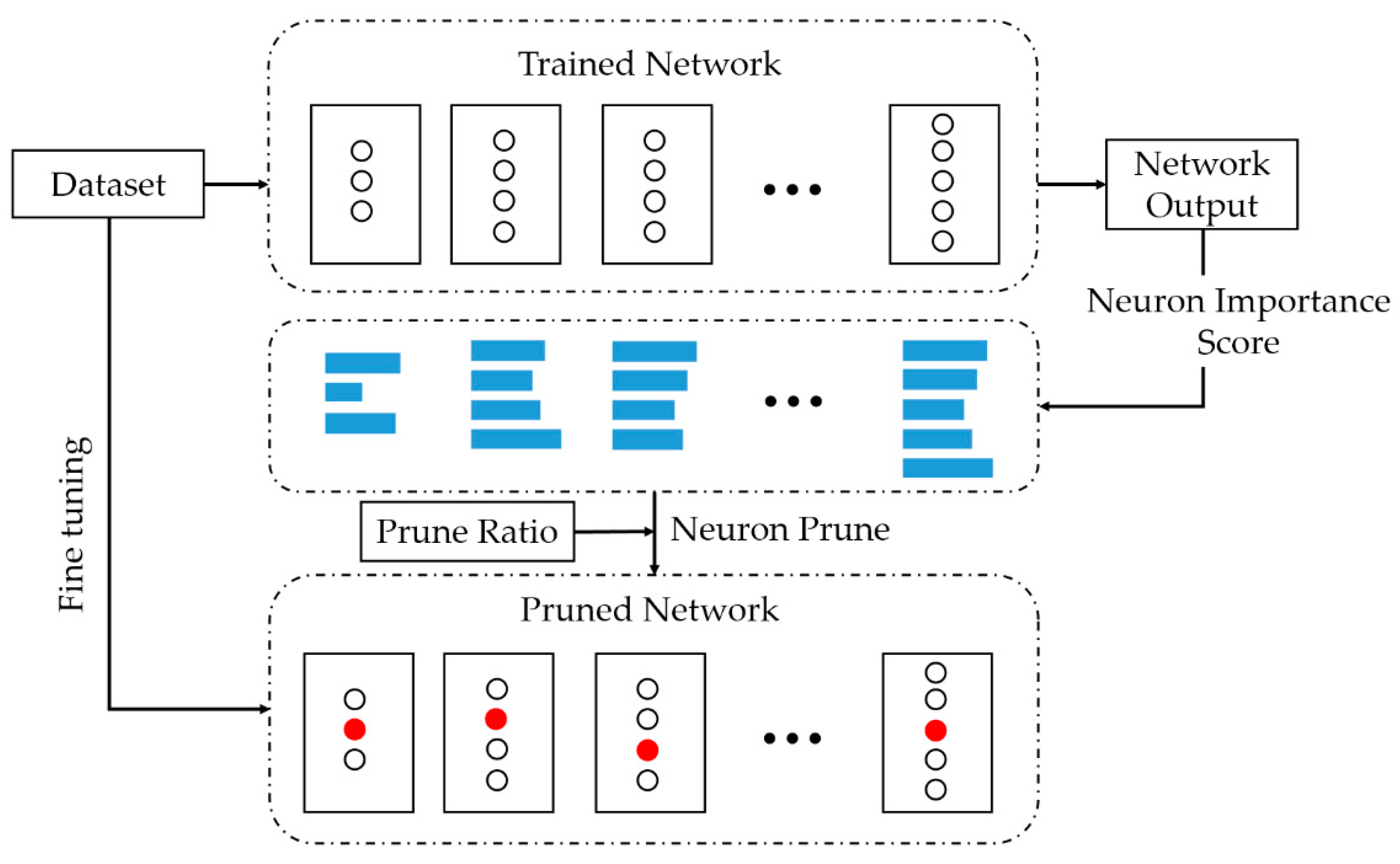
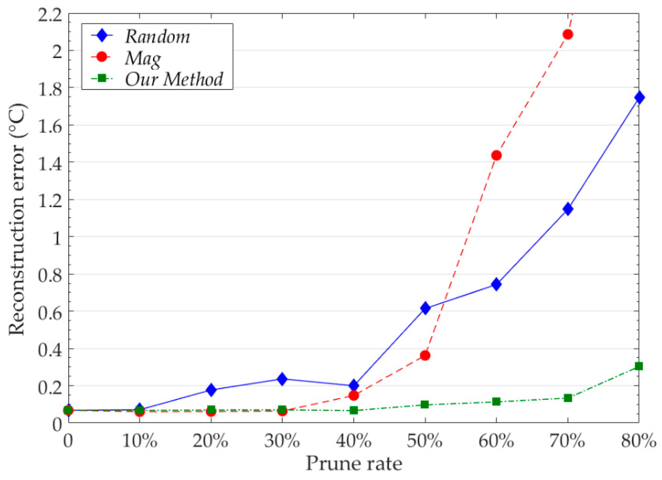
- We proposed a new idea to judge the importance of neural network neurons. We used this idea to guide neural network pruning to further reduce network parameters and computational consumption.
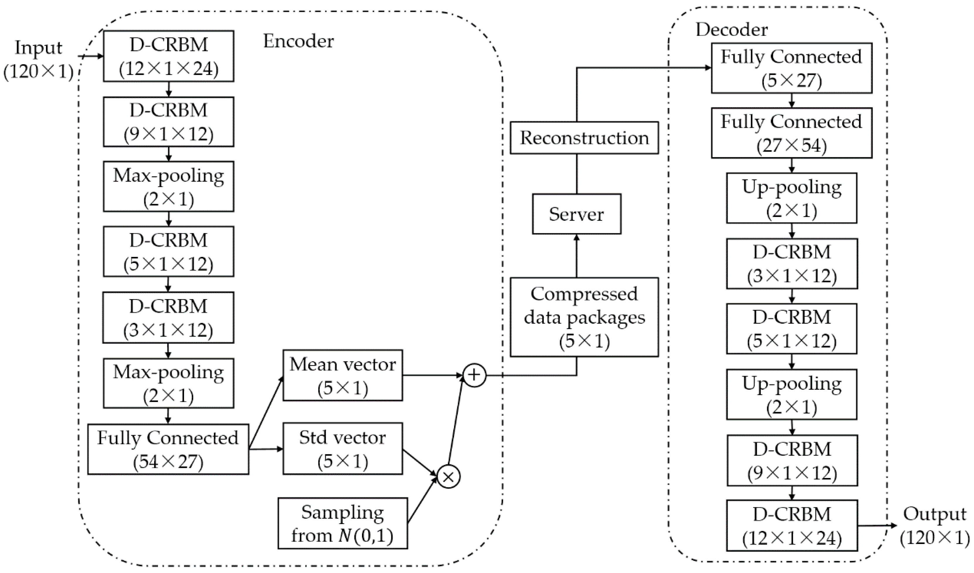
2. CBN-VAE Model Architecture
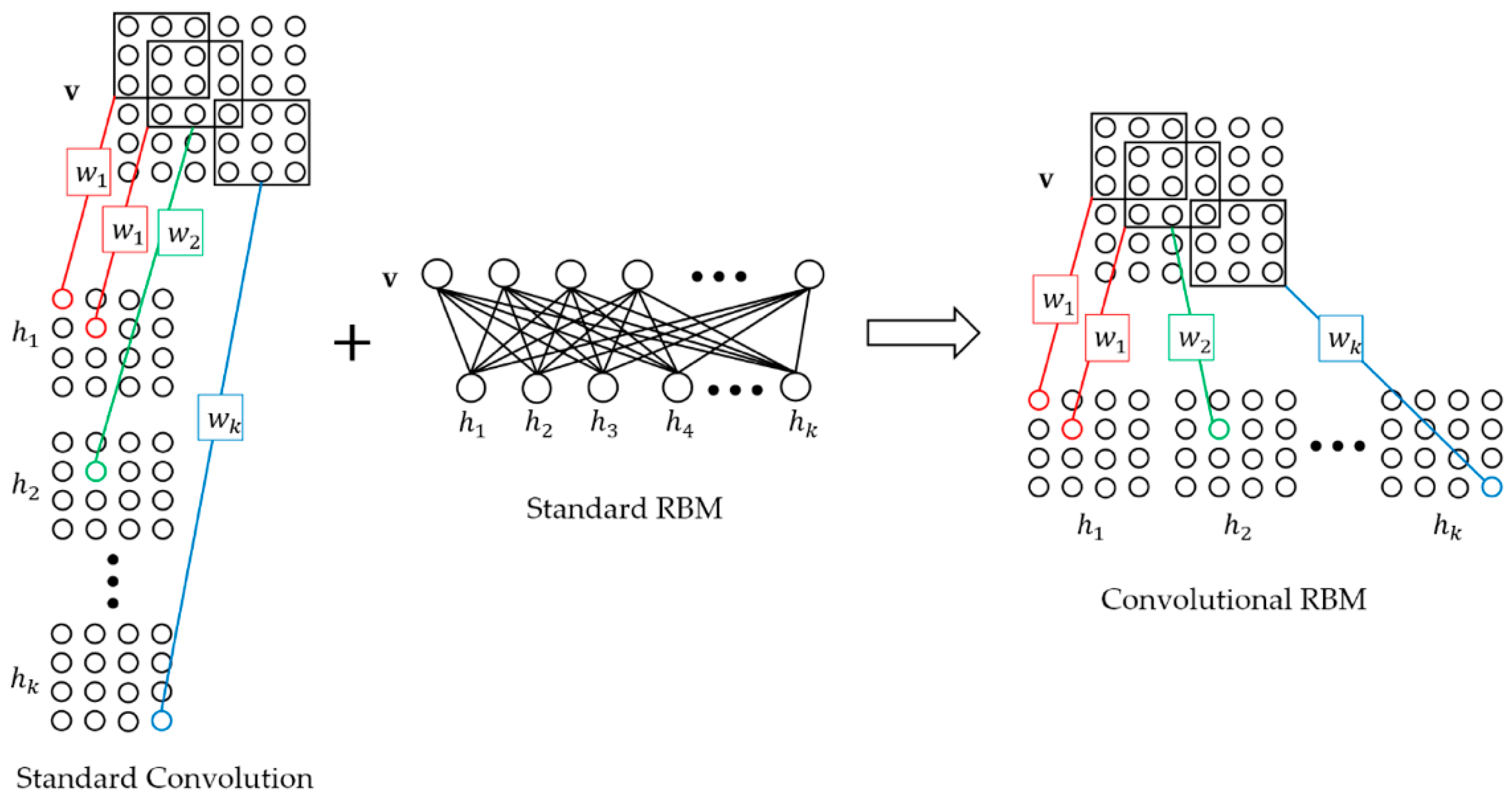
2.1. Downsampling-Convolutional RBM
2.2. Model Structure and Training
- Change the convolution output feature map dimension. This method can significantly reduce the number of convolution kernel parameters for the next convolutional layer. For a convolutional layer with output size of , the parameters of next convolutional layer convolution kernel should be where is the size of kernel and is the number of kernel. After we turn the output to where , the parameters of next convolutional layer convolution kernel should be . Compared with standard convolution, this method can reduce the parameters and computation consumption of in the layer-width.
- Share network parameters. Parameter sharing can be divided into two aspects: one is the parameter sharing of the convolution kernel in the layer-width; and the other is the undirected graph characteristic of D-CRBM, the parameters between the encoder and decoder networks can be shared.
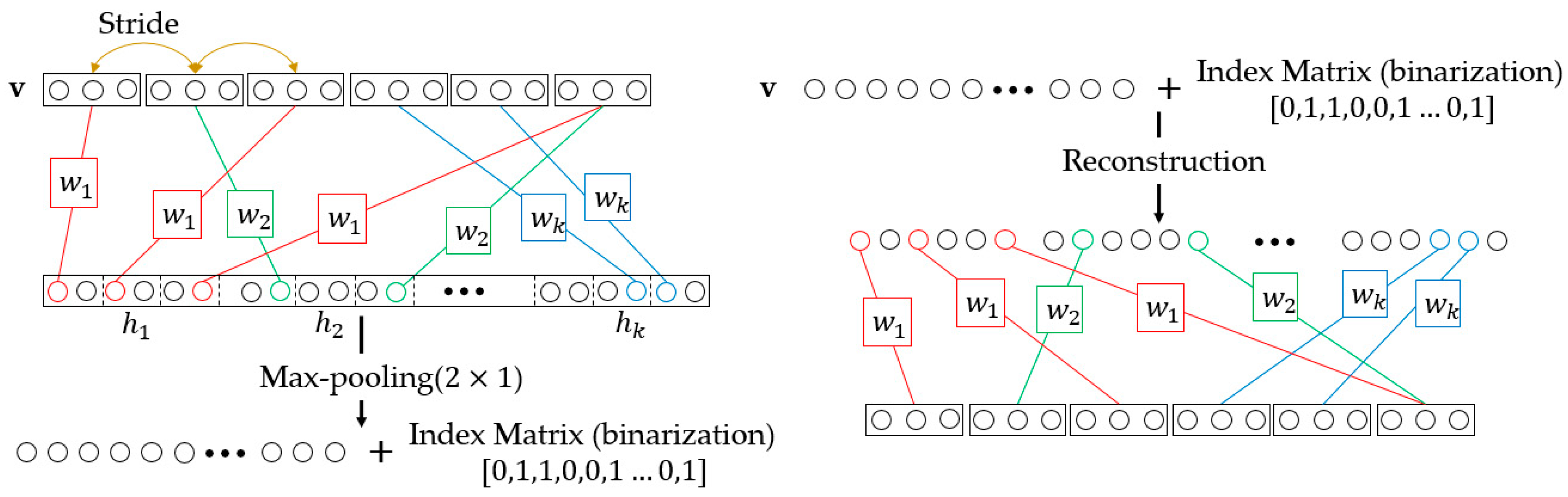
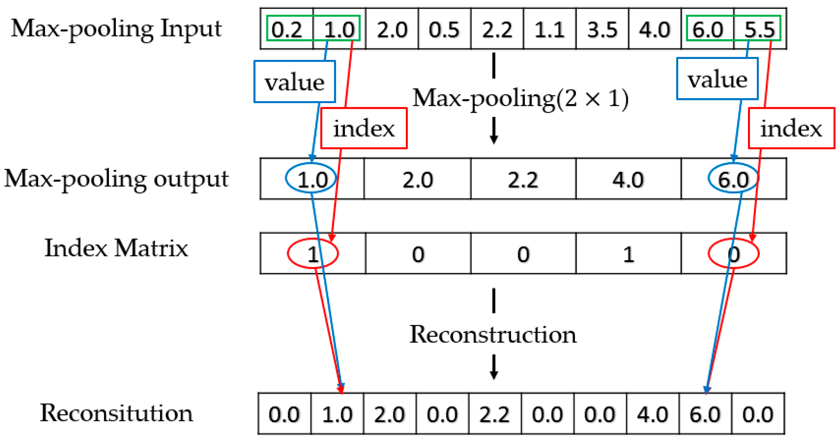
- D-CRBM. Downsampling convolution by using the variable convolution stride and max-pooling. Change the convolution stride can reduce the redundancy caused by the convolution kernel repeated calculation of the same data. The max-pooling operation can further reduce the network redundancy.
| Algorithm 1: Training of the Stacked CBN-VAE model. |
| 1:Input: A mini-batch of training data set S, the number of train iteration iter, the learning rate α |
| 2: While i < iter do |
| 3: Compute the reconstructed output through forward propagation |
| 4: Compute the model loss according to (3) |
| 5: Compute the gradient of parameters according to (4) |
| 6: Update parameters according to (5) |
| 7: i + + |
| 8:end |
3. Experiments
3.1. Dataset Preprocess
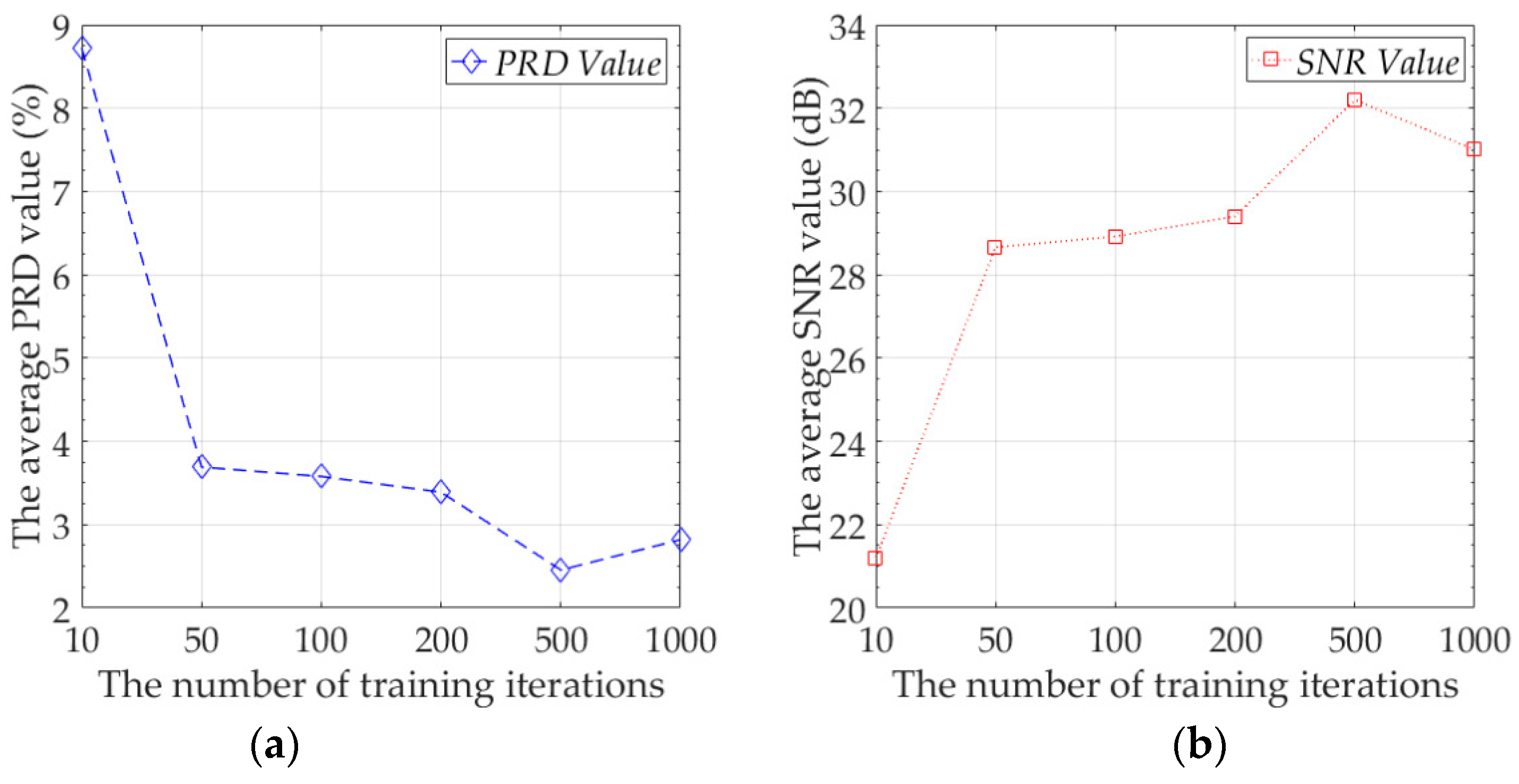
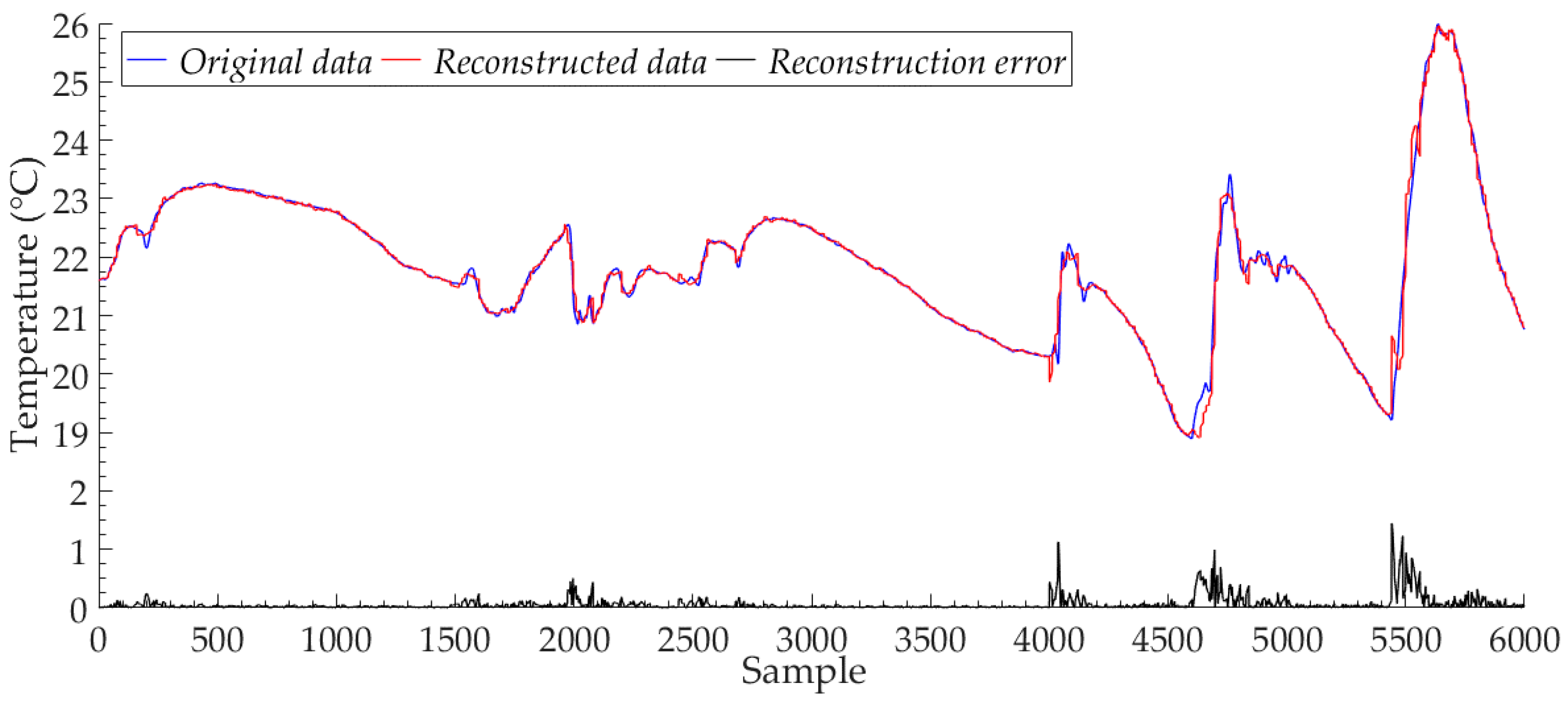
3.2. Compression and Reconstruction
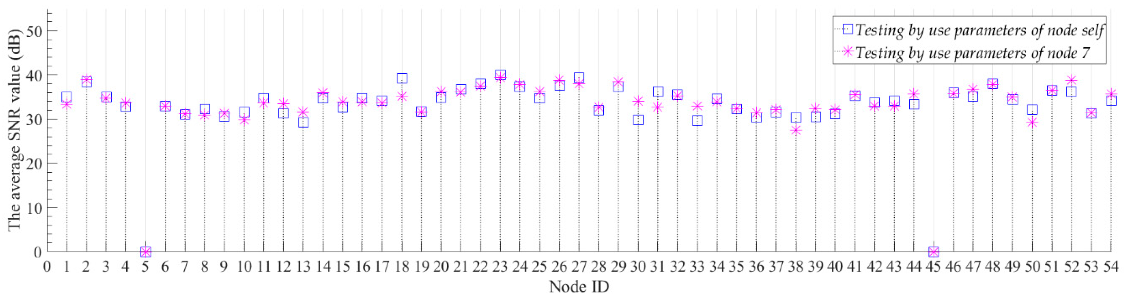
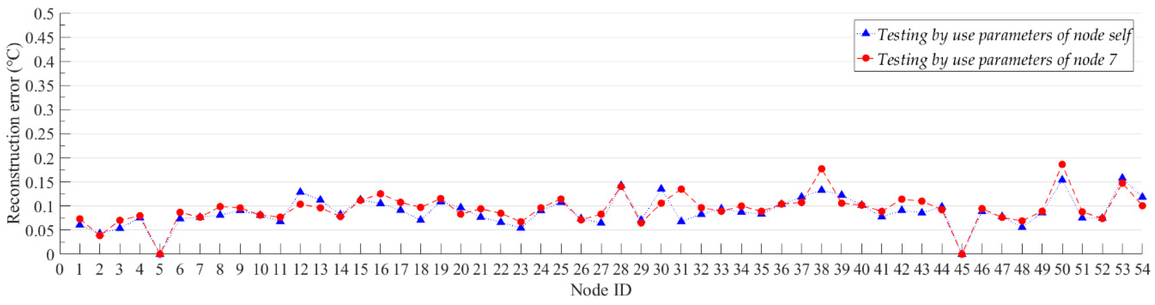
3.3. Transfer Learning
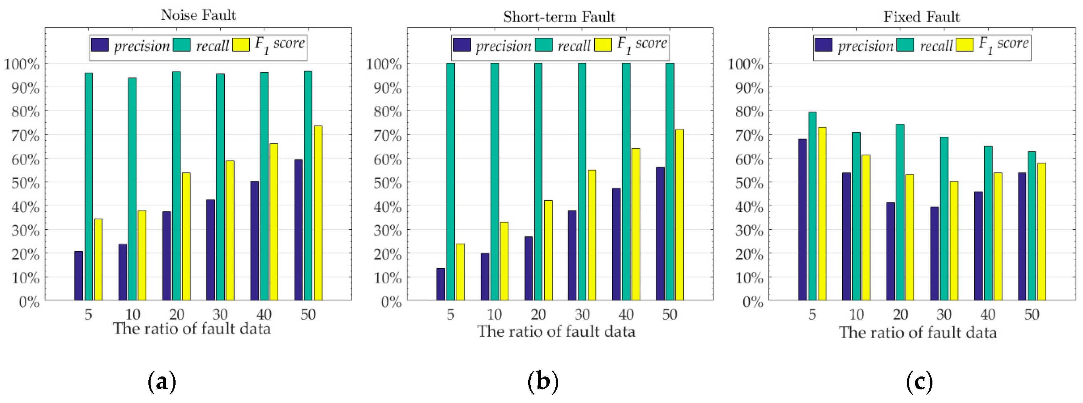
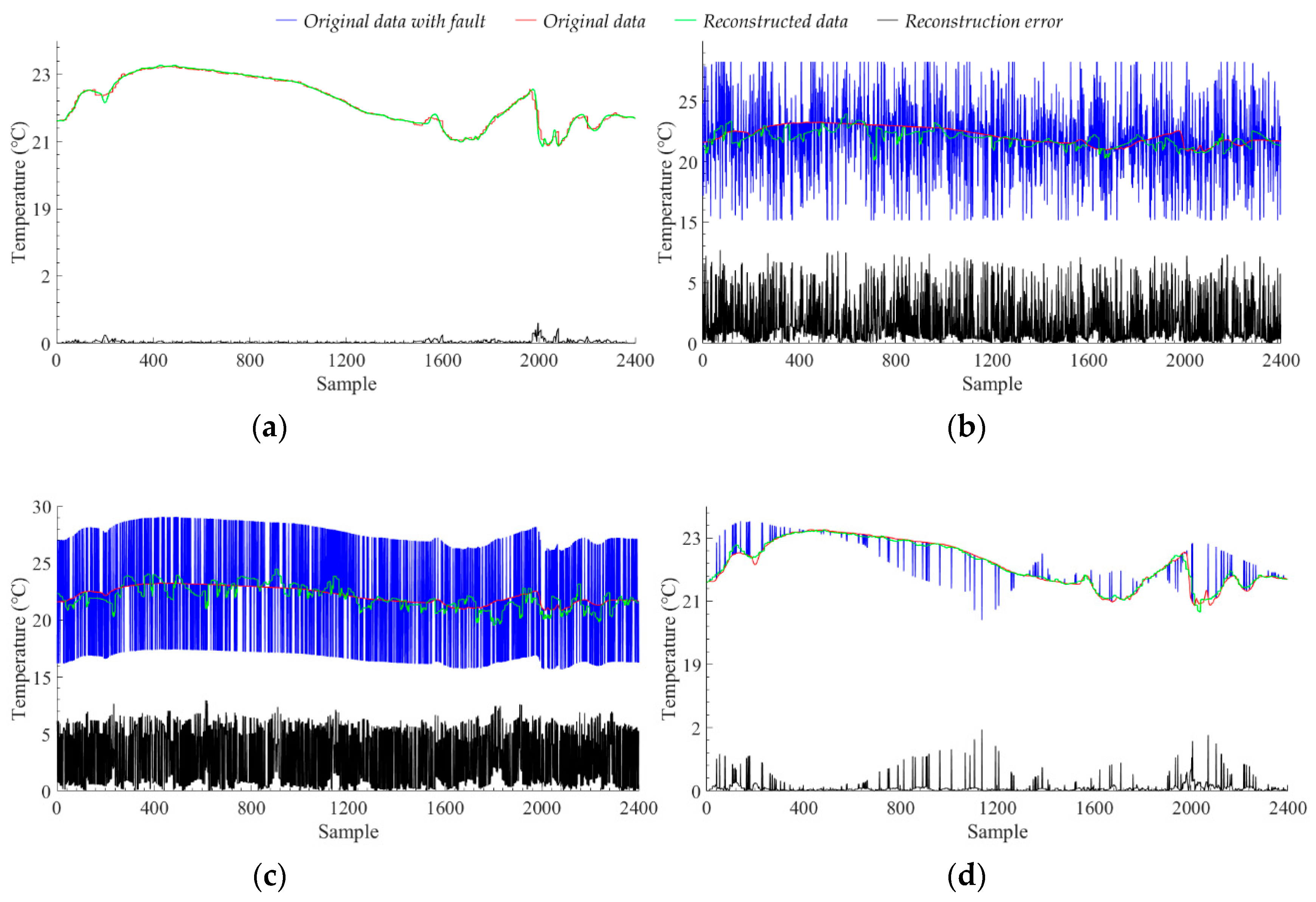
3.4. Fault Detection and Anti-Noise Analysis
3.5. Energy Analysis and Optimization
| Algorithm 2: Pruning Neurons. |
| 1: Input: The model weights W, the prune rate α, the number of prune iterations iter |
| 2: Get which is the number of elements in W |
| 3: Get the number of W that need pruning |
| 4: Calculate the importance of neurons, get the neuron importance score matrix |
| 5: Sorting from large to small |
| 6: Get the prune threshold of neuron importance score |
| 7: While i < m do |
| 8: if < thr then |
| 9: W = 0 |
| 10: end |
| 11: |
| 12: end |
| 13: While k < iter do |
| 14: Retrain the model to update parameters according to Algorithm 1 |
| 15: Execute step 2–12 |
| 16: |
| 17: end |
4. Conclusions
Author Contributions
Funding
Conflicts of Interest
References
- Rawat, P.; Singh, K.D.; Chaouchi, H.; Bonnin, J. Wireless sensor networks: A survey on recent developments and potential synergies. J. Supercomput. 2014, 68, 1–48. [Google Scholar] [CrossRef]
- Venetis, I.E.; Gavalas, D.; Pantziou, G.E.; Konstantopoulos, C. Mobile agents-based data aggregation in WSNs: Benchmarking itinerary planning approaches. Wirel. Netw. 2018, 24, 2111–2132. [Google Scholar] [CrossRef]
- He, S.; Chen, J.; Yau, D.K.Y.; Sun, Y. Cross-Layer Optimization of Correlated Data Gathering in Wireless Sensor Networks. IEEE Trans. Mob. Comput. 2012, 11, 1678–1691. [Google Scholar] [CrossRef]
- Tang, X.; Xie, H.; Chen, W.; Niu, J.; Wang, S. Data Aggregation Based on Overlapping Rate of Sensing Area in Wireless Sensor Networks. Sensors 2017, 17, 1527. [Google Scholar] [CrossRef] [PubMed]
- Sadler, C.M.; Martonosi, M. Data compression algorithms for energy-constrained devices in delay tolerant networks. In Proceedings of the ACM—4th International Conference on Embedded Networked Sensor Systems, Boulder, CO, USA, 1–3 November 2006; pp. 265–278. [Google Scholar]
- Marcelloni, F.; Vecchio, M. A simple algorithm for data compression in wireless sensor networks. IEEE Commun. Lett. 2008, 12, 411–413. [Google Scholar] [CrossRef]
- Tharini, C.; Ranjan, P.V. Design of modified adaptive Huffman data compression algorithm for wireless sensor network. J. Comput. Sci. 2009, 5, 466. [Google Scholar] [CrossRef]
- Săcăleanu, D.I.; Stoian, R.; Ofrim, D.M. An adaptive Huffman algorithm for data compression in wireless sensor networks. In Proceedings of the ISSCS 2011—International Symposium on Signals, Circuits and Systems, Iasi, Romania, 30 June–1 July 2011; IEEE: Piscataway, NJ, USA, 2011; pp. 1–4. [Google Scholar]
- Cao, X.; Madria, S.; Hara, T. A WSN testbed for Z-order encoding based multi-modal sensor data compression. In Proceedings of the 14th Annual IEEE International Conference on Sensing, Communication, and Networking (SECON), San Diego, CA, USA, 12–14 June 2017; IEEE: Piscataway, NJ, USA, 2017; pp. 1–2. [Google Scholar]
- Zordan, D.; Martinez, B.; Vilajosana, I.; Rossi, M. To compress or not to compress: Processing vs transmission tradeoffs for energy constrained sensor networking. Comput. Sci. 2012, 534, 314–322. [Google Scholar]
- Sheltami, T.; Musaddiq, M.; Shakshuki, E. Data compression techniques in wireless sensor networks. Future Gener. Comput. Syst. 2016, 64, 151–162. [Google Scholar] [CrossRef]
- Pham, N.D.; Le, T.D.; Choo, H. Enhance exploring temporal correlation for data collection in WSNs. In Proceedings of the IEEE International Conference on Research, Innovation and Vision for the Future in Computing and Communication Technologies, Ho Chi Minh City, Vietnam, 13–17 July 2008; IEEE: Piscataway, NJ, USA, 2008; pp. 204–208. [Google Scholar]
- Narang, B.; Kaur, A.; Singh, D. Comparison of DWT and DFT for energy efficiency in underwater WSNs. Int. J. Comput. Sci. Mob. Comput. 2015, 4, 128–137. [Google Scholar]
- Shen, G.; Ortega, A. Transform-based distributed data gathering. IEEE Trans. Signal Process. 2010, 58, 3802–3815. [Google Scholar] [CrossRef]
- Schoellhammer, T.; Greenstein, B.; Osterweil, E.; Wimbrow, M.; Estrin, D. Lightweight temporal compression of microclimate datasets. In Proceedings of the 29th Annual IEEE International Conference on Local Computer Networks, Tampa, FL, USA, 16–18 November 2004; IEEE: Piscataway, NJ, USA, 2004. [Google Scholar]
- Marcelloni, F.; Vecchio, M. Enabling energy-efficient and lossy-aware data compression in wireless sensor networks by multi-objective evolutionary optimization. Inf. Sci. 2010, 180, 1924–1941. [Google Scholar] [CrossRef]
- Donoho, D.L. Compressed sensing. IEEE Trans. Inf. Theory. 2006, 52, 1289–1306. [Google Scholar] [CrossRef]
- Milenković, A.; Otto, C.; Jovanov, E. Wireless sensor networks for personal health monitoring: Issues and an implementation. Comput. Commun. 2006, 29, 2521–2533. [Google Scholar] [CrossRef]
- Donoho, D.L.; Tsaig, Y.; Drori, I.; Starck, J.L. Sparse solution of underdetermined systems of linear equations by stagewise orthogonal matching pursuit. IEEE Trans. Inf. Theory 2012, 58, 1094–1121. [Google Scholar] [CrossRef]
- Kingma, D.P.; Welling, M. Auto-encoding variational bayes. arXiv preprint 2013, arXiv:1312.6114. [Google Scholar]
- Salakhutdinov, R.; Mnih, A.; Hinton, G. Restricted Boltzmann machines for collaborative filtering. In Proceedings of the 24th International Conference on Machine Learning, Corvalis, OR, USA, 20–24 June 2007; ACM: New York, NY, USA, 2007; pp. 791–798. [Google Scholar]
- Alsheikh, M.A.; Lin, S.; Niyato, D.; Tan, H.P. Machine learning in wireless sensor networks: Algorithms, strategies, and applications. IEEE Commun. Surv. Tutor. 2014, 16, 1996–2018. [Google Scholar] [CrossRef]
- Wu, M.; Tan, L.; Xiong, N. Data prediction, compression, and recovery in clustered wireless sensor networks for environmental monitoring applications. Inf. Sci. 2016, 329, 800–818. [Google Scholar] [CrossRef]
- Krause, A.; Singh, A.; Guestrin, C. Near-optimal sensor placements in Gaussian processes: Theory, efficient algorithms and empirical studies. J. Mach. Learn. Res. 2008, 9, 235–284. [Google Scholar]
- Masiero, R.; Quer, G.; Munaretto, D.; Rossi, M.; Widmer, J.; Zorzi, M. Data acquisition through joint compressive sensing and principal component analysis. In Proceedings of the GLOBECOM 2009—2009 IEEE Global Telecommunications Conference, Honolulu, HI, USA, 30 November–4 December 2009; IEEE: Piscataway, NJ, USA, 2009; pp. 1–6. [Google Scholar]
- Mousavi, A.; Patel, A.B.; Baraniuk, R.G. A deep learning approach to structured signal recovery. In Proceedings of the 53rd Annual Allerton Conference on Communication, Control, and Computing (Allerton), Monticello, IL, USA, 30 September–2 October 2015; IEEE: Piscataway, NJ, USA, 2015; pp. 1336–1343. [Google Scholar] [Green Version]
- Qiu, L.; Liu, T.J.; Fu, P. Data fusion in wireless sensor network based on sparse filtering. J. Electron. Meas. Instrum. 2015, 3, 352–357. [Google Scholar]
- Alsheikh, A.M.; Poh, P.K.; Lin, S.; Tan, H.P.; Niyato, D. Efficient data compression with error bound guarantee in wireless sensor networks. In Proceedings of the 17th ACM International Conference on Modeling, Analysis and Simulation of Wireless and Mobile Systems, Montreal, QC, Canada, 21–26 September 2014; ACM: New York, NY, USA, 2014; pp. 307–311. [Google Scholar] [Green Version]
- Kumsawat, P.; Attakitmongcol, K.; Srikaew, A. A new optimum signal compression algorithm based on discrete wavelet transform and neural networks For Wsn. In Proceedings of the IAENG Transactions on Engineering Sciences, London, UK, 1–3 July 2015; pp. 118–131. [Google Scholar]
- Liu, J.; Chen, F.; Wang, D. Data Compression Based on Stacked RBM-AE Model for Wireless Sensor Networks. Sensors 2018, 18, 4273. [Google Scholar] [CrossRef]
- Yildirim, O.; San, T.R.; Acharya, U.R. An efficient compression of ECG signals using deep convolutional autoencoders. Cogn. Syst. Res. 2018, 52, 198–211. [Google Scholar] [CrossRef]
- Norouzi, M.; Ranjbar, M.; Mori, G. Stacks of convolutional restricted boltzmann machines for shift-invariant feature learning. In Proceedings of the IEEE Conference on Computer Vision and Pattern Recognition, Miami, FL, USA, 20–25 June 2009; IEEE: Piscataway, NJ, USA, 2009; pp. 2735–2742. [Google Scholar]
- Rumelhart, D.E.; Hinton, G.E.; Williams, R.J. Learning representations by back-propagating errors. Nature 1986, 323, 533. [Google Scholar] [CrossRef]
- Intel Lab Data. Intel Lab Data Homepage. Available online: http://db.csail.mit.edu (accessed on 10 December 2018).
- Argo. Argo Homepage. Available online: http://www.argo.org.cn (accessed on 10 December 2018).
- CRAWDAD. CRAWDAD Homepage. Available online: http://crawdad.org (accessed on 10 December 2018).
- Bottou, L. Large-scale machine learning with stochastic gradient descent. In Proceedings of COMPSTAT’2010; Physica-Verlag HD: Heidelberg/Berlin, Germany, 2010; pp. 177–186. [Google Scholar]
- Kingma, D.P.; Ba, J. Adam: A method for stochastic optimization. arXiv preprint 2014, arXiv:1412.6980. [Google Scholar]
- Takianngam, S.; Usaha, W. Discrete Wavelet Transform and One-Class Support Vector Machines for anomaly detection in wireless sensor networks. In Proceedings of the International Symposium on Intelligent Signal, Processing and Communications Systems (ISPACS), Chiang Mai, Thailand, 7–9 December 2011; IEEE: Piscataway, NJ, USA, 2011; pp. 1–6. [Google Scholar]
- Howard, A.G.; Zhu, M.; Chen, B.; Kalenichenko, D.; Wang, W.; Weyand, T.; Andreetto, M.; Adam, H. MobileNets: Efficient Convolutional Neural Networks for Mobile Vision Applications. arXiv preprint 2017, arXiv:1704.04861. [Google Scholar]


| No | Layer Name | Kernel Size | Activation Function | No. of Parameters | Output Size |
|---|---|---|---|---|---|
| Encoder | |||||
| 1 | D-CRBM | 12 × 1 × 24 | ReLU | 312 | 120 × 1 × 1 |
| 2 | D-CRBM | 9 × 1 × 12 | ReLU | 120 | 84 × 1 × 1 |
| 3 | Max-pooling (2 × 1) | 42 × 1 × 1 | |||
| 4 | D-CRBM | 5 × 1 × 12 | ReLU | 72 | 54 × 1 × 1 |
| 5 | D-CRBM | 3 × 1 × 12 | ReLU | 48 | 108 × 1 × 1 |
| 6 | Max-pooling (2 × 1) | 54 × 1 × 1 | |||
| 7 | Fully Connected | 54 × 27 | ReLU | 1485 | 27 × 1 |
| 8 | Fully Connected | 27 × 5 | ReLU | 140 | 5 × 1 |
| 9 | Fully Connected | 27 × 5 | ReLU | 140 | 5 × 1 |
| Decoder | |||||
| 10 | Fully Connected | 5 × 27 | ReLU | 140 | 27 × 1 |
| 11 | Fully Connected | 27 × 54 | ReLU | 1485 | 54 × 1 × 1 |
| 12 | Up-pooling (2 × 1) | 108 × 1 × 1 | |||
| 13 | D-CRBM | 3 × 1 × 12 | ReLU | 48 | 54 × 1 × 1 |
| 14 | D-CRBM | 5 × 1 × 12 | ReLU | 72 | 42 × 1 × 1 |
| 15 | Up-pooling (2 × 1) | 84 × 1 × 1 | |||
| 16 | D-CRBM | 9 × 1 × 12 | ReLU | 120 | 120 × 1 × 1 |
| 17 | D-CRBM | 12 × 1 × 24 | ReLU | 312 | 120 × 1 × 1 |
| Algorithm | CR | PRD (%) | SNR (dB) | Reconstruction Error (°C) |
|---|---|---|---|---|
| CS | 10 | 38.40 | 8.31 | 1.4143 |
| LTC | 13.93 | 8.45 | 21.46 | 0.2904 |
| DPCM-o | 13.85 | 8.00 | 21.94 | 0.2342 |
| Stacked RBM-AE | 10 | 10.04 | 19.97 | 0.2815 |
| Stacked RBM-VAE | 24 | 9.49 | 20.45 | 0.2926 |
| CNN-AE | 24 | 3.80 | 28.39 | 0.1075 |
| CBN-VAE | 24 | 2.37 | 32.51 | 0.0678 |
| CBN-VAE-b | 10 | 1.70 | 35.40 | 0.0454 |
| CBN-VAE-c | 40 | 2.52 | 31.98 | 0.0770 |
| Dataset | CR | PRD (%) | SNR (dB) | Reconstruction Error |
|---|---|---|---|---|
| Argo (temperature) | 24 | 1.18 | 38.56 | 0.0984 (°C) |
| ZebraNet (location/UTM format) | 24 | 7.23 | 22.82 | 114.22 |
| CRAWDAD (speed) | 24 | 2.02 | 33.89 | 1.0897 (km/h) |
| IBRL (voltage) | 24 | 6.61 | 23.58 | 0.0199 (V) |
| IBRL (humidity) | 24 | 4.04 | 27.85 | 0.5096 (%RH) |
| Model | FLOPs | No. of Parameters | CP-Time (ms) | FP-Time (ms) | TR-Time (ms) |
|---|---|---|---|---|---|
| Stacked RBM-AE | 35,850 | 19,032 | 0.2113 | 0.3873 | 1.0211 |
| Stacked RBM-VAE | 36,150 | 19,234 | 0.2817 | 0.4577 | 1.6549 |
| CNN-AE | 772,008 | 9245 | 0.9859 | 1.5493 | 2.6761 |
| CBN-VAE | 27,564 | 2415 | 0.1761 | 1.162 | 1.7606 |
© 2019 by the authors. Licensee MDPI, Basel, Switzerland. This article is an open access article distributed under the terms and conditions of the Creative Commons Attribution (CC BY) license (http://creativecommons.org/licenses/by/4.0/).
Share and Cite
Liu, J.; Chen, F.; Yan, J.; Wang, D. CBN-VAE: A Data Compression Model with Efficient Convolutional Structure for Wireless Sensor Networks. Sensors 2019, 19, 3445. https://doi.org/10.3390/s19163445
Liu J, Chen F, Yan J, Wang D. CBN-VAE: A Data Compression Model with Efficient Convolutional Structure for Wireless Sensor Networks. Sensors. 2019; 19(16):3445. https://doi.org/10.3390/s19163445
Chicago/Turabian StyleLiu, Jianlin, Fenxiong Chen, Jun Yan, and Dianhong Wang. 2019. "CBN-VAE: A Data Compression Model with Efficient Convolutional Structure for Wireless Sensor Networks" Sensors 19, no. 16: 3445. https://doi.org/10.3390/s19163445
APA StyleLiu, J., Chen, F., Yan, J., & Wang, D. (2019). CBN-VAE: A Data Compression Model with Efficient Convolutional Structure for Wireless Sensor Networks. Sensors, 19(16), 3445. https://doi.org/10.3390/s19163445