A Novel Swarm Intelligence—Harris Hawks Optimization for Spatial Assessment of Landslide Susceptibility

 , ,
, ,  ,
,  , and
, and
Abstract
:1. Introduction
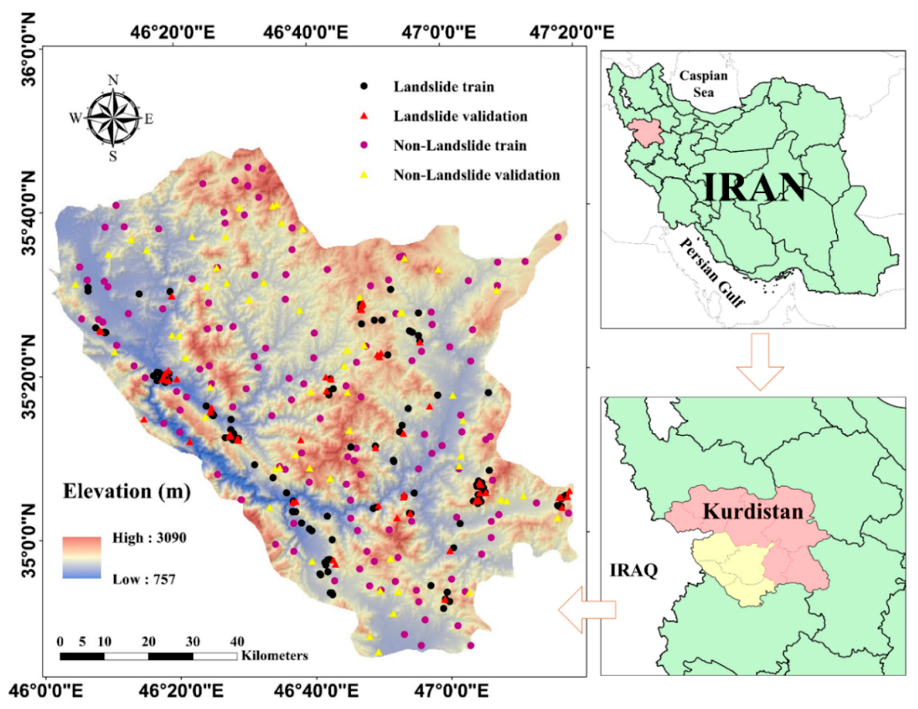
2. Study Area
3. Data Preparation and Spatial Relationship between the Landslide and Related Factors
4. Methodology
4.1. Artificial Neural Network
4.2. Harris Hawks Optimization
5. Results and Discussion
5.1. Model Implementation
5.2. Landslide Susceptibility Mapping
5.3. Performance Assessment of the Models
5.4. Presenting the HHO-Based Predictive Formula
0.3330 × Z3 + 0.1148 × Z4 + 0.4546 × Z5 + 0.5011 × Z6 − 0.6282 ×
Z7 + 0.6683 × Z8 − 0.3576,
6. Conclusions
Author Contributions
Funding
Acknowledgments
Conflicts of Interest
Appendix A
References
- Varnes, D.J.; Radbruch-Hall, D.H. Landslides cause and effect. Bull. Int. Assoc. Eng. Geol 1976, 13, 205–216. [Google Scholar]
- Cruden, D.M. A simple definition of a landslide. Bull. Eng. Geol. Environ. 1991, 43, 27–29. [Google Scholar] [CrossRef]
- Fell, R.; Corominas, J.; Bonnard, C.; Cascini, L.; Leroi, E.; Savage, W.Z. Guidelines for landslide susceptibility, hazard and risk zoning for land-use planning. Eng. Geol. 2008, 102, 99–111. [Google Scholar] [CrossRef] [Green Version]
- Pourghasemi, H.R.; Pradhan, B.; Gokceoglu, C. Application of fuzzy logic and analytical hierarchy process (AHP) to landslide susceptibility mapping at Haraz watershed, Iran. Nat. Hazards 2012, 63, 965–996. [Google Scholar] [CrossRef]
- Shoaei, Z.; Ghayoumian, J. The largest debris flow in the world, Seimareh Landslide, Western Iran. In Environmental Forest Science; Springer: Dordrecht, The Netherlands, 1998; pp. 553–561. [Google Scholar]
- Hong, H.; Miao, Y.; Liu, J.; Zhu, A.X. Exploring the effects of the design and quantity of absence data on the performance of random forest-based landslide susceptibility mapping. Catena 2019, 176, 45–64. [Google Scholar] [CrossRef]
- Ercanoglu, M.; Gokceoglu, C. Use of fuzzy relations to produce landslide susceptibility map of a landslide prone area (West Black Sea Region, Turkey). Eng. Geol. 2004, 75, 229–250. [Google Scholar] [CrossRef]
- Song, Y.; Gong, J.; Gao, S.; Wang, D.; Cui, T.; Li, Y.; Wei, B. Susceptibility assessment of earthquake-induced landslides using Bayesian network: A case study in Beichuan, China. Comput. Geosci. 2012, 42, 189–199. [Google Scholar] [CrossRef]
- Pradhan, B. A comparative study on the predictive ability of the decision tree, support vector machine and neuro-fuzzy models in landslide susceptibility mapping using GIS. Comput. Geosci. 2013, 51, 350–365. [Google Scholar] [CrossRef]
- Chen, W.; Chai, H.; Sun, X.; Wang, Q.; Ding, X.; Hong, H. A GIS-based comparative study of frequency ratio, statistical index and weights-of-evidence models in landslide susceptibility mapping. Arab. J. Geosci. 2016, 9, 204. [Google Scholar] [CrossRef]
- Nicu, I.C. Application of analytic hierarchy process, frequency ratio, and statistical index to landslide susceptibility: An approach to endangered cultural heritage. Environ. Earth Sci. 2018, 77, 79. [Google Scholar] [CrossRef]
- Razavizadeh, S.; Solaimani, K.; Massironi, M.; Kavian, A. Mapping landslide susceptibility with frequency ratio, statistical index, and weights of evidence models: a case study in northern Iran. Environ. Earth Sci. 2017, 76, 499. [Google Scholar] [CrossRef]
- Youssef, A.M.; Al-Kathery, M.; Pradhan, B. Landslide susceptibility mapping at Al-Hasher area, Jizan (Saudi Arabia) using GIS-based frequency ratio and index of entropy models. Geosci. J. 2015, 19, 113–134. [Google Scholar] [CrossRef]
- Chen, W.; Pourghasemi, H.R.; Naghibi, S.A. A comparative study of landslide susceptibility maps produced using support vector machine with different kernel functions and entropy data mining models in China. Bull. Eng. Geol. Environ. 2018, 77, 647–664. [Google Scholar] [CrossRef]
- Vahidnia, M.H.; Alesheikh, A.A.; Alimohammadi, A.; Hosseinali, F. A GIS-based neuro-fuzzy procedure for integrating knowledge and data in landslide susceptibility mapping. Comput. Geosci. 2010, 36, 1101–1114. [Google Scholar] [CrossRef]
- Chen, W.; Yan, X.; Zhao, Z.; Hong, H.; Bui, D.T.; Pradhan, B. Spatial prediction of landslide susceptibility using data mining-based kernel logistic regression, naive Bayes and RBFNetwork models for the Long County area (China). Bull. Eng. Geol. Environ. 2019, 78, 247–266. [Google Scholar] [CrossRef]
- Oh, H.J.; Pradhan, B. Application of a neuro-fuzzy model to landslide-susceptibility mapping for shallow landslides in a tropical hilly area. Comput. Geosci. 2011, 37, 1264–1276. [Google Scholar] [CrossRef]
- Pradhan, B.; Lee, S.; Buchroithner, M.F. A GIS-based back-propagation neural network model and its cross-application and validation for landslide susceptibility analyses. Comput. Environ. Urban Syst. 2010, 34, 216–235. [Google Scholar] [CrossRef]
- Tian, Y.; Xu, C.; Hong, H.; Zhou, Q.; Wang, D. Mapping earthquake-triggered landslide susceptibility by use of artificial neural network (ANN) models: an example of the 2013 Minxian (China) Mw 5.9 event. Geomat. Nat. Hazards Risk 2019, 10, 1–25. [Google Scholar] [CrossRef]
- Yilmaz, I. Landslide susceptibility mapping using frequency ratio, logistic regression, artificial neural networks and their comparison: a case study from Kat landslides (Tokat-Turkey). Comput. Geosci. 2009, 35, 1125–1138. [Google Scholar] [CrossRef]
- Pham, B.T.; Bui, D.T.; Pourghasemi, H.R.; Indra, P.; Dholakia, M. Landslide susceptibility assesssment in the Uttarakhand area (India) using GIS: a comparison study of prediction capability of naïve bayes, multilayer perceptron neural networks, and functional trees methods. Theor. Appl. Climatol. 2017, 128, 255–273. [Google Scholar] [CrossRef]
- Bui, D.T.; Tuan, T.A.; Klempe, H.; Pradhan, B.; Revhaug, I. Spatial prediction models for shallow landslide hazards: a comparative assessment of the efficacy of support vector machines, artificial neural networks, kernel logistic regression, and logistic model tree. Landslides 2016, 13, 361–378. [Google Scholar]
- Chen, W.; Panahi, M.; Pourghasemi, H.R. Performance evaluation of GIS-based new ensemble data mining techniques of adaptive neuro-fuzzy inference system (ANFIS) with genetic algorithm (GA), differential evolution (DE), and particle swarm optimization (PSO) for landslide spatial modelling. Catena 2017, 157, 310–324. [Google Scholar] [CrossRef]
- Bui, D.T.; Tuan, T.A.; Hoang, N.D.; Thanh, N.Q.; Nguyen, D.B.; Van Liem, N.; Pradhan, B. Spatial prediction of rainfall-induced landslides for the Lao Cai area (Vietnam) using a hybrid intelligent approach of least squares support vector machines inference model and artificial bee colony optimization. Landslides 2017, 14, 447–458. [Google Scholar]
- Jaafari, A.; Panahi, M.; Pham, B.T.; Shahabi, H.; Bui, D.T.; Rezaie, F.; Lee, S. Meta optimization of an adaptive neuro-fuzzy inference system with grey wolf optimizer and biogeography-based optimization algorithms for spatial prediction of landslide susceptibility. Catena 2019, 175, 430–445. [Google Scholar] [CrossRef]
- Zhang, T.; Han, L.; Chen, W.; Shahabi, H. Hybrid integration approach of entropy with logistic regression and support vector machine for landslide susceptibility modeling. Entropy 2018, 20, 884. [Google Scholar] [CrossRef]
- Tien Bui, D.; Shahabi, H.; Shirzadi, A.; Chapi, K.; Hoang, N.D.; Pham, B.; Bui, Q.T.; Tran, C.T.; Panahi, M.; Bin Ahamd, B. A novel integrated approach of relevance vector machine optimized by imperialist competitive algorithm for spatial modeling of shallow landslides. Remote Sens. 2018, 10, 1538. [Google Scholar] [CrossRef]
- Xi, W.; Li, G.; Moayedi, H.; Nguyen, H. A particle-based optimization of artificial neural network for earthquake-induced landslide assessment in Ludian county, China. Geomat. Nat. Hazards Risk 2019, 10, 1750–1771. [Google Scholar] [CrossRef] [Green Version]
- Gao, W.; Guirao, J.L.G.; Basavanagoud, B.; Wu, J. Partial multi-dividing ontology learning algorithm. Inf. Sci. 2018, 467, 35–58. [Google Scholar] [CrossRef]
- Gao, W.; Wang, W.; Dimitrov, D.; Wang, Y. Nano properties analysis via fourth multiplicative ABC indicator calculating. Arab. J. Chem. 2018, 11, 793–801. [Google Scholar] [CrossRef]
- Gao, W.; Wu, H.; Siddiqui, M.K.; Baig, A.Q. Study of biological networks using graph theory. Saudi J. Biol. Sci. 2018, 25, 1212–1219. [Google Scholar] [CrossRef]
- Moayedi, H.; Mehrabi, M.; Mosallanezhad, M.; Rashid, A.S.A.; Pradhan, B. Modification of landslide susceptibility mapping using optimized PSO-ANN technique. Eng. Comput. 2018, 35, 1–18. [Google Scholar] [CrossRef]
- Nguyen, H.; Mehrabi, M.; Kalantar, B.; Moayedi, H.; Abdullahi, M.M. Potential of hybrid evolutionary approaches for assessment of geo-hazard landslide susceptibility mapping. Geomat. Nat. Hazards Risk 2019, 10, 1667–1693. [Google Scholar] [CrossRef]
- Shirzadi, A.; Chapi, K.; Shahabi, H.; Solaimani, K.; Kavian, A.; Ahmad, B.B. Rock fall susceptibility assessment along a mountainous road: an evaluation of bivariate statistic, analytical hierarchy process and frequency ratio. Environ. Earth Sci. 2017, 76, 152. [Google Scholar] [CrossRef]
- Rahmati, O.; Samani, A.N.; Mahdavi, M.; Pourghasemi, H.R.; Zeinivand, H. Groundwater potential mapping at Kurdistan region of Iran using analytic hierarchy process and GIS. Arab. J. Geosci. 2015, 8, 7059–7071. [Google Scholar] [CrossRef]
- Pourghasemi, H.R.; Kerle, N. Random forests and evidential belief function-based landslide susceptibility assessment in Western Mazandaran Province, Iran. Environ. Earth Sci. 2016, 75, 185. [Google Scholar] [CrossRef]
- Ercanoglu, M.; Gokceoglu, C. Assessment of landslide susceptibility for a landslide-prone area (north of Yenice, NW Turkey) by fuzzy approach. Environ. Geol. 2002, 41, 720–730. [Google Scholar]
- Talebi, A.; Uijlenhoet, R.; Troch, P.A. Soil moisture storage and hillslope stability. Nat. Hazards Earth Syst. Sci. 2007, 7, 523–534. [Google Scholar] [CrossRef] [Green Version]
- Vakhshoori, V.; Pourghasemi, H.R. A novel hybrid bivariate statistical method entitled FROC for landslide susceptibility assessment. Environ. Earth Sci. 2018, 77, 686. [Google Scholar] [CrossRef]
- Oh, H.J.; Kim, Y.S.; Choi, J.K.; Park, E.; Lee, S. GIS mapping of regional probabilistic groundwater potential in the area of Pohang City, Korea. J. Hydrol. 2011, 399, 158–172. [Google Scholar] [CrossRef]
- McCulloch, W.S.; Pitts, W. A logical calculus of the ideas immanent in nervous activity. Bull. Math. Biophys. 1943, 5, 115–133. [Google Scholar] [CrossRef]
- ASCE Task Committee Artificial neural networks in hydrology. II: Hydrologic applications. J. Hydrol. Eng. 2000, 5, 124–137. [CrossRef]
- Moayedi, H.; Hayati, S. Modelling and optimization of ultimate bearing capacity of strip footing near a slope by soft computing methods. Appl. Soft Comput. 2018, 66, 208–219. [Google Scholar] [CrossRef]
- Moayedi, H.; Huat, B.B.; Mohammad Ali, T.A.; Asadi, A.; Moayedi, F.; Mokhberi, M. Preventing landslides in times of rainfall: case study and FEM analyses. Disaster Prev. Manage. Int. J. 2011, 20, 115–124. [Google Scholar] [CrossRef] [Green Version]
- Moayedi, H.; Rezaei, A. An artificial neural network approach for under-reamed piles subjected to uplift forces in dry sand. Neural Comput. Appl. 2019, 31, 327–336. [Google Scholar] [CrossRef]
- Moayedi, H.; Hayati, S. Applicability of a CPT-Based Neural Network Solution in Predicting Load-Settlement Responses of Bored Pile. Int. J. Geomech. 2018, 18, 06018009. [Google Scholar] [CrossRef]
- Seyedashraf, O.; Mehrabi, M.; Akhtari, A.A. Novel approach for dam break flow modeling using computational intelligence. J. Hydrol. 2018, 559, 1028–1038. [Google Scholar] [CrossRef]
- Heidari, A.A.; Mirjalili, S.; Faris, H.; Aljarah, I.; Mafarja, M.; Chen, H. Harris Hawks optimization: Algorithm and applications. Future Gener. Comput. Syst. 2019, 97, 849–872. [Google Scholar] [CrossRef]
- Moayedi, H.; Osouli, A.; Nguyen, H.; Rashid, A.S.A. A novel Harris hawks’ optimization and k-fold cross-validation predicting slope stability. Eng. Comput. 2019, 1–11. [Google Scholar] [CrossRef]
- Ayalew, L.; Yamagishi, H.; Ugawa, N. Landslide susceptibility mapping using GIS-based weighted linear combination, the case in Tsugawa area of Agano River, Niigata Prefecture, Japan. Landslides 2004, 1, 73–81. [Google Scholar] [CrossRef]
- Tehrany, M.S.; Jones, S.; Shabani, F.; Martínez-Álvarez, F.; Bui, D.T. A novel ensemble modeling approach for the spatial prediction of tropical forest fire susceptibility using logitboost machine learning classifier and multi-source geospatial data. Theor. Appl. Climatol. 2019, 137, 637–653. [Google Scholar] [CrossRef]
- Liu, J.; Duan, Z. Quantitative assessment of landslide susceptibility comparing statistical index, index of entropy, and weights of evidence in the Shangnan area, China. Entropy 2018, 20, 868. [Google Scholar] [CrossRef]
- Jenks, G.F. The data model concept in statistical mapping. Int. Yearb. Cartogr. 1967, 7, 186–190. [Google Scholar]
- Irigaray, C.; Fernández, T.; El Hamdouni, R.; Chacón, J. Evaluation and validation of landslide-susceptibility maps obtained by a GIS matrix method: examples from the Betic Cordillera (southern Spain). Nat. Hazards 2007, 41, 61–79. [Google Scholar] [CrossRef]
- Pourghasemi, H.R.; Pradhan, B.; Gokceoglu, C.; Moezzi, K.D. A comparative assessment of prediction capabilities of Dempster—Shafer and weights-of-evidence models in landslide susceptibility mapping using GIS. Geomat. Nat. Hazards Risk 2013, 4, 93–118. [Google Scholar] [CrossRef]
- Xu, C.; Dai, F.; Xu, X.; Lee, Y.H. GIS-based support vector machine modeling of earthquake-triggered landslide susceptibility in the Jianjiang River watershed, China. Geomorphology 2012, 145, 70–80. [Google Scholar] [CrossRef]
- Akgun, A.; Sezer, E.A.; Nefeslioglu, H.A.; Gokceoglu, C.; Pradhan, B. An easy-to-use MATLAB program (MamLand) for the assessment of landslide susceptibility using a Mamdani fuzzy algorithm. Comput. Geosci. 2012, 38, 23–34. [Google Scholar] [CrossRef]
- Jaafari, A.; Najafi, A.; Pourghasemi, H.; Rezaeian, J.; Sattarian, A. GIS-based frequency ratio and index of entropy models for landslide susceptibility assessment in the Caspian forest, northern Iran. Int. J. Environ. Sci. Technol. 2014, 11, 909–926. [Google Scholar] [CrossRef] [Green Version]
- Swets, J.A. Measuring the accuracy of diagnostic systems. Science 1988, 240, 1285–1293. [Google Scholar] [CrossRef]
- Lasko, T.A.; Bhagwat, J.G.; Zou, K.H.; Ohno-Machado, L. The use of receiver operating characteristic curves in biomedical informatics. J. Biomed. Inf. 2005, 38, 404–415. [Google Scholar] [CrossRef] [Green Version]
- Beguería, S. Validation and evaluation of predictive models in hazard assessment and risk management. Nat. Hazards 2006, 37, 315–329. [Google Scholar] [CrossRef]
- Hanley, J.A.; McNeil, B.J. A method of comparing the areas under receiver operating characteristic curves derived from the same cases. Radiology 1983, 148, 839–843. [Google Scholar] [CrossRef]
- Lee, S.; Ryu, J.H.; Won, J.S.; Park, H.J. Determination and application of the weights for landslide susceptibility mapping using an artificial neural network. Eng. Geol. 2004, 71, 289–302. [Google Scholar] [CrossRef]
- Can, A.; Dagdelenler, G.; Ercanoglu, M.; Sonmez, H. Landslide susceptibility mapping at Ovacık-Karabük (Turkey) using different artificial neural network models: comparison of training algorithms. Bull. Eng. Geol. Environ. 2019, 78, 89–102. [Google Scholar] [CrossRef]
- Chen, W.; Pourghasemi, H.R.; Panahi, M.; Kornejady, A.; Wang, J.; Xie, X.; Cao, S. Spatial prediction of landslide susceptibility using an adaptive neuro-fuzzy inference system combined with frequency ratio, generalized additive model, and support vector machine techniques. Geomorphology 2017, 297, 69–85. [Google Scholar] [CrossRef]
- Bui, D.T.; Bui, Q.T.; Nguyen, Q.P.; Pradhan, B.; Nampak, H.; Trinh, P.T. A hybrid artificial intelligence approach using GIS-based neural-fuzzy inference system and particle swarm optimization for forest fire susceptibility modeling at a tropical area. Agric. For. Meteorol. 2017, 233, 32–44. [Google Scholar]
- Bui, Q.T. Metaheuristic algorithms in optimizing neural network: a comparative study for forest fire susceptibility mapping in Dak Nong, Vietnam. Geomat. Nat. Hazards Risk 2019, 10, 136–150. [Google Scholar] [CrossRef]
- Chen, W.; Tsangaratos, P.; Ilia, I.; Duan, Z.; Chen, X. Groundwater spring potential mapping using population-based evolutionary algorithms and data mining methods. Sci. Total Environ. 2019, 684, 31–49. [Google Scholar] [CrossRef]
- Khosravi, K.; Panahi, M.; Bui, D.T. Spatial Prediction of Groundwater Spring Potential Mapping Based on Adaptive Neuro-Fuzzy Inference System and Metaheuristic Optimization. Hydrol. Earth Syst. Sci. 2018, 22, 1–22. [Google Scholar] [CrossRef]
- Pradhan, B.; Lee, S. Regional landslide susceptibility analysis using back-propagation neural network model at Cameron Highland, Malaysia. Landslides 2010, 7, 13–30. [Google Scholar] [CrossRef]
- Du, P.; Wang, J.; Hao, Y.; Niu, T.; Yang, W. A novel hybrid model based on multi-objective Harris hawks optimization algorithm for daily PM2. 5 and PM10 forecasting. arXiv 2019, arXiv:1905.13550. [Google Scholar]


| Symbol | Description | Age | Age Era | FR |
|---|---|---|---|---|
| Qft1 | High level piedmont fan and valley terrace deposits | Quaternary | Cenozoic | 0.32 |
| OMql | Massive to thick-bedded reefal limestone | Oligocene–Miocene | Cenozoic | 5.94 |
| pCmt1 | Medium grade, regional metamorphic rocks (Amphibolite Facies) | Pre-Cambrian | Proterozoic | 0.00 |
| Kav | Andesitic volcanic | Late Cretaceous | Mesozoic | 0.00 |
| Kfsh | Dark grey argillaceous shale | Cretaceous | Mesozoic | 0.11 |
| K1m | Limestone, argillaceous limestone, tile red sandstone and gypsiferous marl | Early Cretaceous | Mesozoic | 0.00 |
| Plms | Marl, shale, sandstone and conglomerate | Pliocene | Cenozoic | 0.00 |
| Klsm | Marl, shale, sandy limestone and sandy dolomite | Early Cretaceous | Mesozoic | 2.20 |
| Qft2 | Low level piedmont fan and valley terrace deposits | Quaternary | Cenozoic | 0.45 |
| E2l | Nummulitic limestone | Eocene | Cenozoic | 0.00 |
| Klsol | Grey thick-bedded to massive orbitolina limestone | Early Cretaceous | Mesozoic | 0.95 |
| K2av | Andesitic volcanic | Late Cretaceous | Mesozoic | 0.00 |
| Murm | Light red to brown marl and gypsiferous marl with sandstone intercalations | Miocene | Cenozoic | 5.74 |
| Pd | Red sandstone and shale with subordinate sandy limestone (Dorud FM) | Permian | Paleozoic | 0.84 |
| Qal | Stream channel, braided channel, and flood plain deposits | Quaternary | Cenozoic | 0.00 |
| PAgr | Granite | Paleocene–Eocene | Cenozoic | 0.00 |
| TRKurl | Purple and red thin-bedded radiolarian chert with intercalations of neritic and pelagic limestone (Kerman and Neyzar radiolarites) | Triassic–Cretaceous | Mesozoic | 0.00 |
| Kussh | Dark grey shale (Sanandaj shale) (Schist and phyllite) | Late Cretaceous | Mesozoic | 1.24 |
| Olc,s | Conglomerate and sandstone | Oligocene | Cenozoic | 6.83 |
| Ebv | Basaltic volcanic rocks | Middle Eocene | Cenozoic | 3.75 |
| Odi-gb | Diorite to gabbro | Oligocene | Cenozoic | 0.00 |
| PeEf | Flysch turbidite, sandstone and calcareous mudstone | Paleocene–Eocene | Cenozoic | 1.83 |
| Qcf | Clay flat | Quaternary | Cenozoic | 0.22 |
| Kupl | Globotruncana limestone | Late Cretaceous | Mesozoic | 0.73 |
| K2l1 | Hyporite bearing limestone (Senonian) | Late Cretaceous | Mesozoic | 0.00 |
| KPef | Thinly bedded sandstone and shale with siltstone, mudstone limestone and conglomerate | Late Cretaceous–Paleocene | Mesozoic–Cenozoic | 0.98 |
| TRKubl | Kuhe Bistoon limestone | Triassic–Cretaceous | Mesozoic | 0.85 |
| Oat | Andesitic tuff | Oligocene | Cenozoic | 0.89 |
| Pel | Medium to thick-bedded limestone | Paleocene–Eocene | Cenozoic | 2.30 |
| TRJvm | Meta-volcanics, phyllites, slate and meta- limestone | Triassic–Jurassic | Mesozoic | 0.00 |
| JKl | Crystalized limestone and calc-schist | Jurassic–Cretaceous | Mesozoic | 0.00 |
| Kbv | Basaltic volcanic | Early Cretaceous | Mesozoic | 0.00 |
| Jugr | Upper Jurassic granite including Shir Kuh granite and Shah Kuh granite | Late Jurassic | Mesozoic | 10.90 |
| Ogb | Gabbro | Oligocene | Cenozoic | 0.34 |
| OMrb | Red beds composed of red conglomerate, sandstone, marl, gypsiferous marl and gypsum | Oligocene–Miocene | Cenozoic | 0.71 |
| pd2 | Peridotite including harzburgite, dunite, lherzolite, and websterite | Triassic–Cretaceous | Mesozoic | 1.02 |
| E1f | Silty shale, sandstone, marl, sandy limestone, limestone and conglomerate | Early Eocene | Cenozoic | 0.88 |
| db | Diabase | Late Cretaceous | Mesozoic | 0.00 |
| sr | Serpentinite | Triassic–Cretaceous | Mesozoic | 0.00 |
| E1l | Nummulitic limestone | Eocene | Cenozoic | 0.00 |
| Methods | Area | Std. Error | p Value | Youden Index j | Asymptotic 95% Confidence Interval | |
|---|---|---|---|---|---|---|
| Lower Bound | Upper Bound | |||||
| ANN | 0.720 | 0.046 | <0.0001 | 0.3710 | 0.630 | 0.809 |
| HHO–ANN | 0.773 | 0.027 | <0.0001 | 0.4247 | 0.720 | 0.826 |
| Susceptibility Class | ANN | HHO–ANN | ||
|---|---|---|---|---|
| Ratio (%) | Area (km2) | Ratio (%) | Area (km2) | |
| Very low | 5.12 | 400.15 | 5.19 | 405.59 |
| Low | 12.36 | 965.71 | 15.27 | 1192.42 |
| Moderate | 25.23 | 1971.09 | 25.64 | 2002.93 |
| High | 33.42 | 2610.36 | 31.96 | 2496.24 |
| Very high | 23.86 | 1864.13 | 21.95 | 1714.26 |
| High and Very high | 57.28 | 4474.50 | 53.90 | 4210.50 |
| Susceptibility Class | ANN | HHO–ANN | ||
|---|---|---|---|---|
| Train | Test | Train | Test | |
| Very low | 1.32 | 1.75 | 1.52 | 1.24 |
| Low | 6.94 | 8.76 | 4.66 | 6.39 |
| Moderate | 21.01 | 20.62 | 15.59 | 16.39 |
| High | 43.14 | 48.76 | 38.89 | 35.98 |
| Very high | 27.59 | 20.10 | 39.34 | 40.00 |
| High and Very high | 70.73 | 68.87 | 78.23 | 75.98 |
| Neurons (i) | Zi = Tansig (Wi1 × Elevation + Wi2 × Slope Degree + Wi3 × Profile Curvature + Wi4 × Plan Curvature + Wi5 × Slope Aspect + Wi6 × SPI + Wi7 × TWI + Wi8 × Land Cover + Wi9 × Rainfall + Wi10 × Lithology + Wi11 × Soil Type + Wi12 × DTT Road + Wi13 × DTT Fault + Wi14 × DTT River + bi) | ||||||||||||||
|---|---|---|---|---|---|---|---|---|---|---|---|---|---|---|---|
| Wi1 | Wi2 | Wi3 | Wi4 | Wi5 | Wi6 | Wi7 | Wi8 | Wi9 | Wi10 | Wi11 | Wi12 | Wi13 | Wi14 | bi | |
| 1 | 0.1389 | 0.8873 | −0.3536 | −0.5390 | 0.6093 | 0.5324 | −0.1268 | −0.2768 | −0.4110 | −0.3422 | −0.2914 | −0.3273 | −0.0984 | 0.6987 | −1.8520 |
| 2 | 0.1941 | −1.1906 | −1.0853 | 0.8015 | 0.0674 | −0.8543 | 0.4639 | −0.3317 | −0.5433 | 0.5304 | −1.0774 | −0.9195 | 0.6389 | −0.6643 | 0.4390 |
| 3 | −0.8748 | 0.1018 | 0.9202 | −0.4856 | −1.0795 | 0.5776 | 0.9880 | 0.8675 | −1.1525 | −0.0134 | 0.5032 | −0.4689 | −1.0977 | 0.0411 | 0.9416 |
| 4 | 0.6930 | 1.0847 | 0.3555 | −0.0661 | 0.4444 | 0.9255 | −1.2186 | 0.1724 | 0.0116 | −1.1188 | 1.3439 | 0.6624 | 0.2156 | 1.0617 | −1.3524 |
| 5 | −0.6105 | −0.0710 | 0.5563 | −2.1150 | 1.2181 | 0.2868 | 0.6106 | 0.0989 | −0.0542 | 0.7688 | −0.3673 | −0.8785 | 1.3454 | −0.1275 | −0.7786 |
| 6 | 0.4460 | −0.4059 | −0.5671 | 0.3063 | −0.2774 | 0.4887 | −0.6989 | −0.3011 | 0.4759 | −0.1634 | −1.0011 | 0.3701 | −0.1290 | −0.8039 | 0.2600 |
| 7 | 0.1713 | −0.7522 | 0.4283 | 0.079 | 0.5879 | 0.4686 | 0.5622 | −0.3228 | 1.2865 | −0.5585 | −0.5446 | 0.5838 | 1.0550 | 0.4543 | 0.5437 |
| 8 | −1.9718 | 0.6761 | −0.5493 | −0.1083 | 0.6430 | −0.6932 | −0.2789 | −0.9709 | 0.9544 | −0.2919 | −0.2008 | −0.0433 | −0.3142 | 1.6938 | −1.3263 |
© 2019 by the authors. Licensee MDPI, Basel, Switzerland. This article is an open access article distributed under the terms and conditions of the Creative Commons Attribution (CC BY) license (http://creativecommons.org/licenses/by/4.0/).
Share and Cite
Bui, D.T.; Moayedi, H.; Kalantar, B.; Osouli, A.; Pradhan, B.; Nguyen, H.; Rashid, A.S.A. A Novel Swarm Intelligence—Harris Hawks Optimization for Spatial Assessment of Landslide Susceptibility. Sensors 2019, 19, 3590. https://doi.org/10.3390/s19163590
Bui DT, Moayedi H, Kalantar B, Osouli A, Pradhan B, Nguyen H, Rashid ASA. A Novel Swarm Intelligence—Harris Hawks Optimization for Spatial Assessment of Landslide Susceptibility. Sensors. 2019; 19(16):3590. https://doi.org/10.3390/s19163590
Chicago/Turabian StyleBui, Dieu Tien, Hossein Moayedi, Bahareh Kalantar, Abdolreza Osouli, Biswajeet Pradhan, Hoang Nguyen, and Ahmad Safuan A Rashid. 2019. "A Novel Swarm Intelligence—Harris Hawks Optimization for Spatial Assessment of Landslide Susceptibility" Sensors 19, no. 16: 3590. https://doi.org/10.3390/s19163590