Author Contributions
Conceptualization, B.O., G.S. and A.F.; Data curation, B.O., G.R. and A.M.; Formal analysis, B.O., G.S., G.R. and A.M.; Investigation, B.O., G.S. and G.R.; Methodology, B.O., G.S., G.R. and A.F.; Supervision, B.O., G.S. and A.F.; Visualization, B.O., G.R. and A.M.; Writing–original draft, B.O. and G.R.; Writing–review & editing, B.O., G.S., G.R., A.M. and A.F.
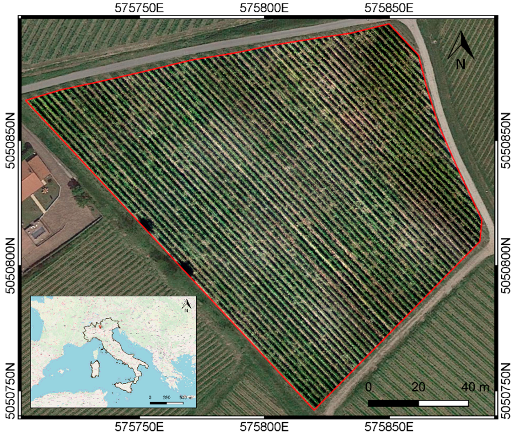
Figure 1.
The experimental site; Coordinate Reference System (CRS): WGS84/UTM zone 32 N. Map data: ©OpenStreetMap contributors.
Figure 1.
The experimental site; Coordinate Reference System (CRS): WGS84/UTM zone 32 N. Map data: ©OpenStreetMap contributors.
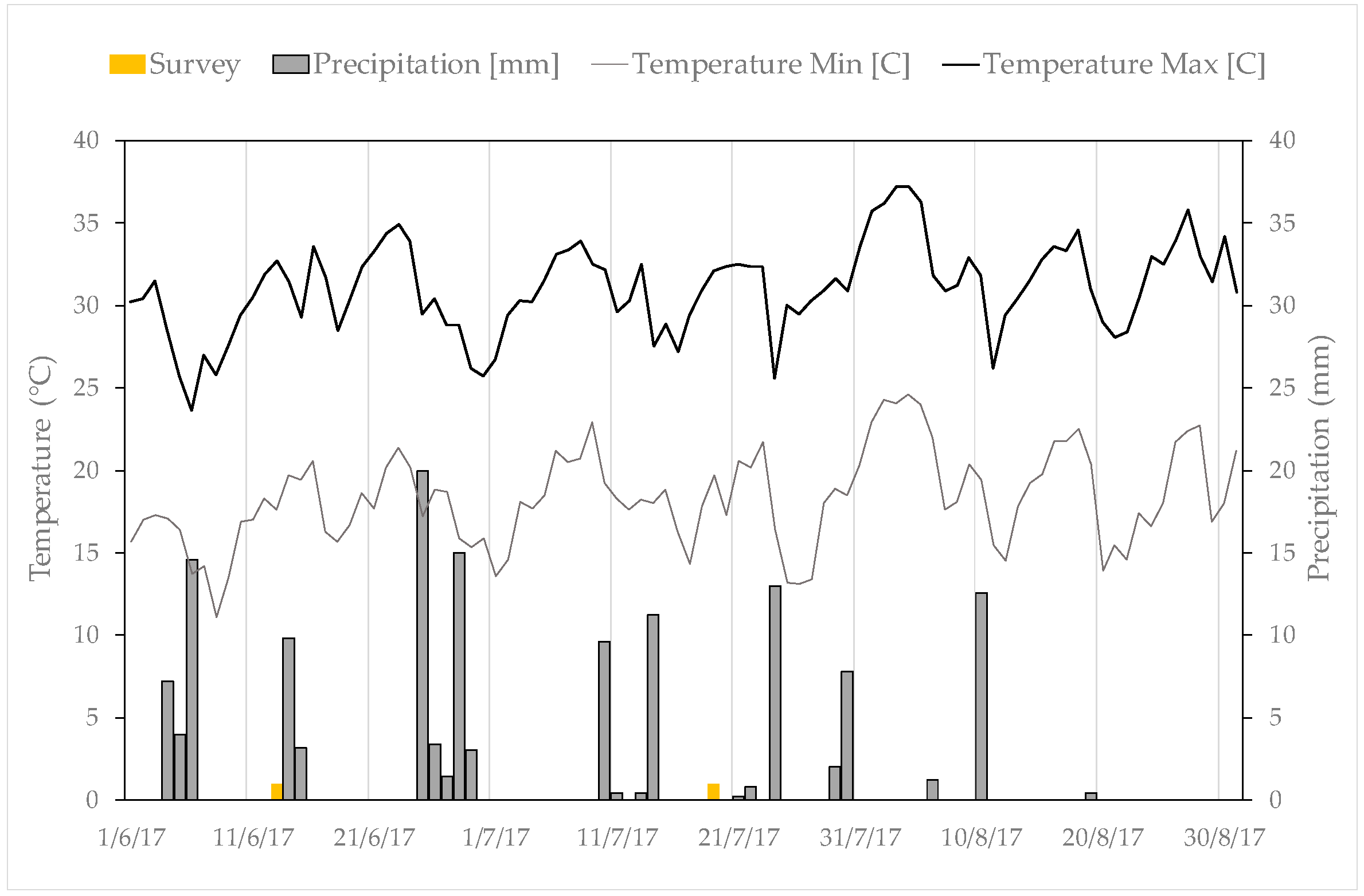
Figure 2.
Precipitation and temperature daily data collected at the agrometeorological station of Erbusco, during the experimental period from June to August 2017.
Figure 2.
Precipitation and temperature daily data collected at the agrometeorological station of Erbusco, during the experimental period from June to August 2017.
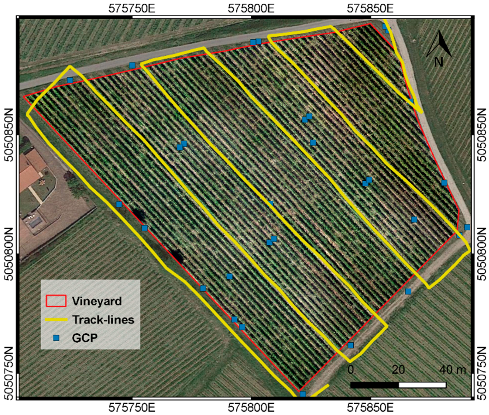
Figure 3.
Flight track-lines for multispectral images acquisition and Ground Control Points (GCPs) distribution. Map data: ©Google Satellite.
Figure 3.
Flight track-lines for multispectral images acquisition and Ground Control Points (GCPs) distribution. Map data: ©Google Satellite.
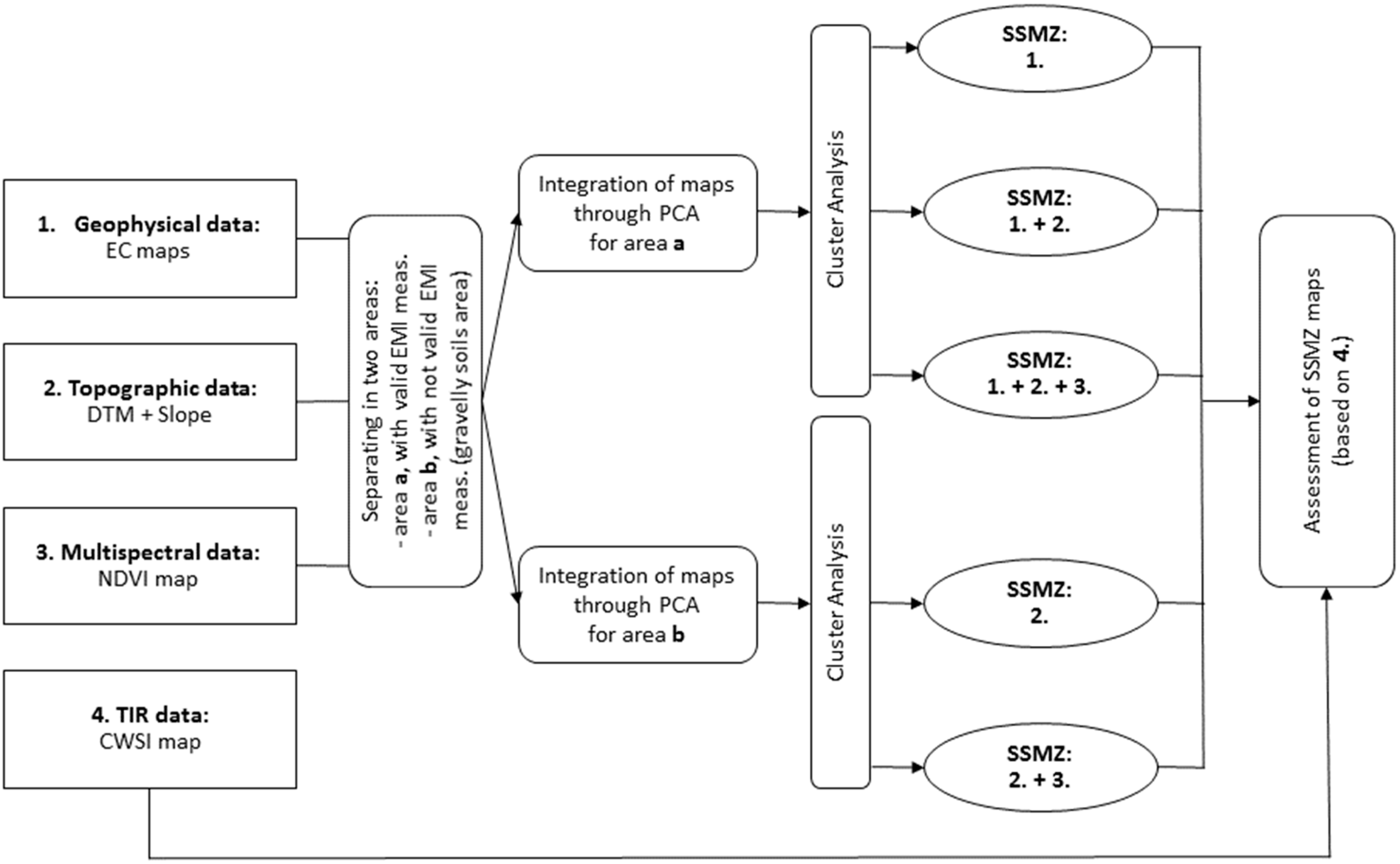
Figure 4.
Scheme of the methodological approach adopted in this study.
Figure 4.
Scheme of the methodological approach adopted in this study.
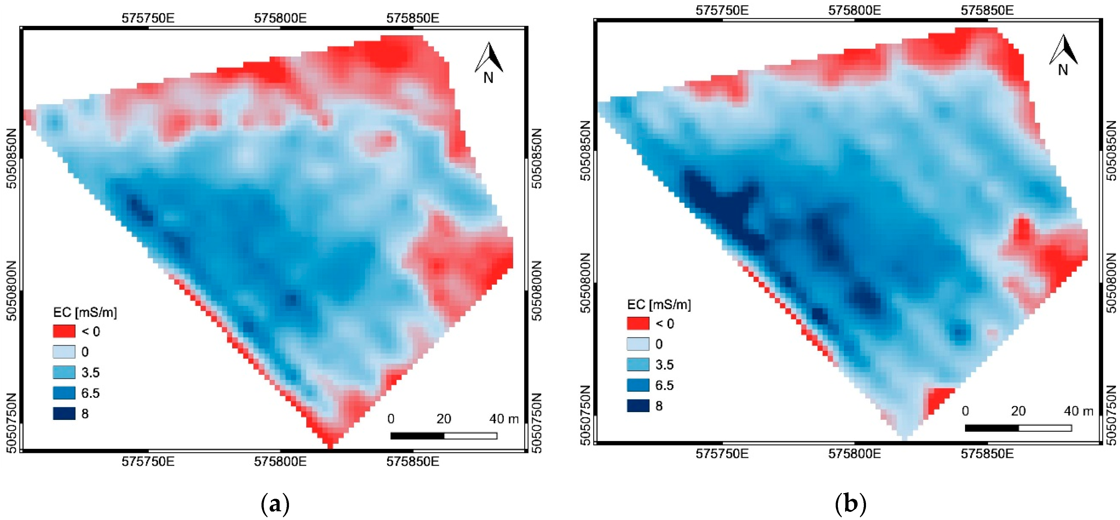
Figure 5.
The obtained EC maps (mS/m): (a) frequency 15 kHz, corresponding to a DoE of 1.5 m; (b) frequency 10 kHz, corresponding to a DoE of 2.5 m. Red color area (area ‘b’) corresponds to gravelly soils (EMI measurement not valid).
Figure 5.
The obtained EC maps (mS/m): (a) frequency 15 kHz, corresponding to a DoE of 1.5 m; (b) frequency 10 kHz, corresponding to a DoE of 2.5 m. Red color area (area ‘b’) corresponds to gravelly soils (EMI measurement not valid).
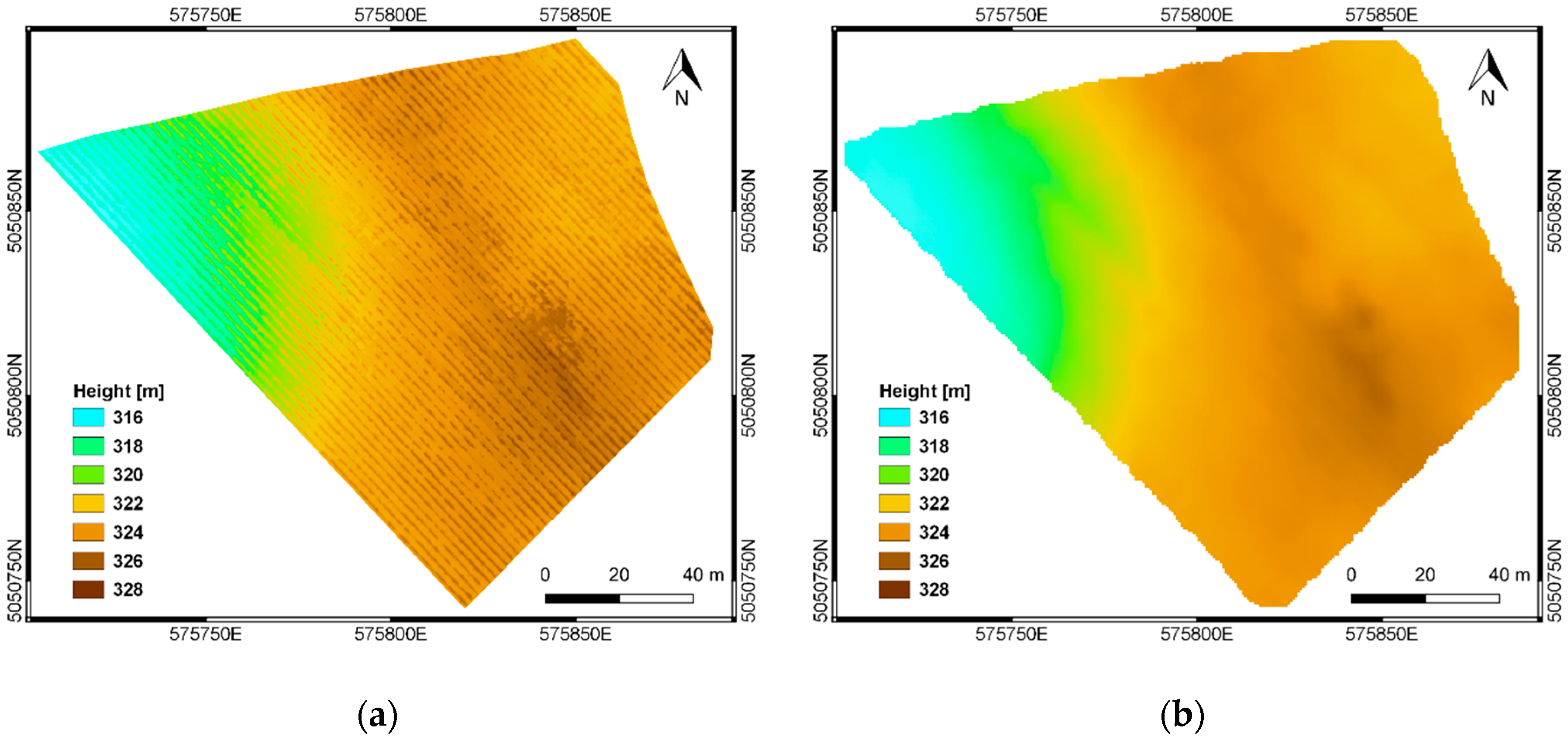
Figure 6.
DSM (a) and DTM (b) produced through photogrammetric processing of multispectral (VIS-NIR) dataset.
Figure 6.
DSM (a) and DTM (b) produced through photogrammetric processing of multispectral (VIS-NIR) dataset.
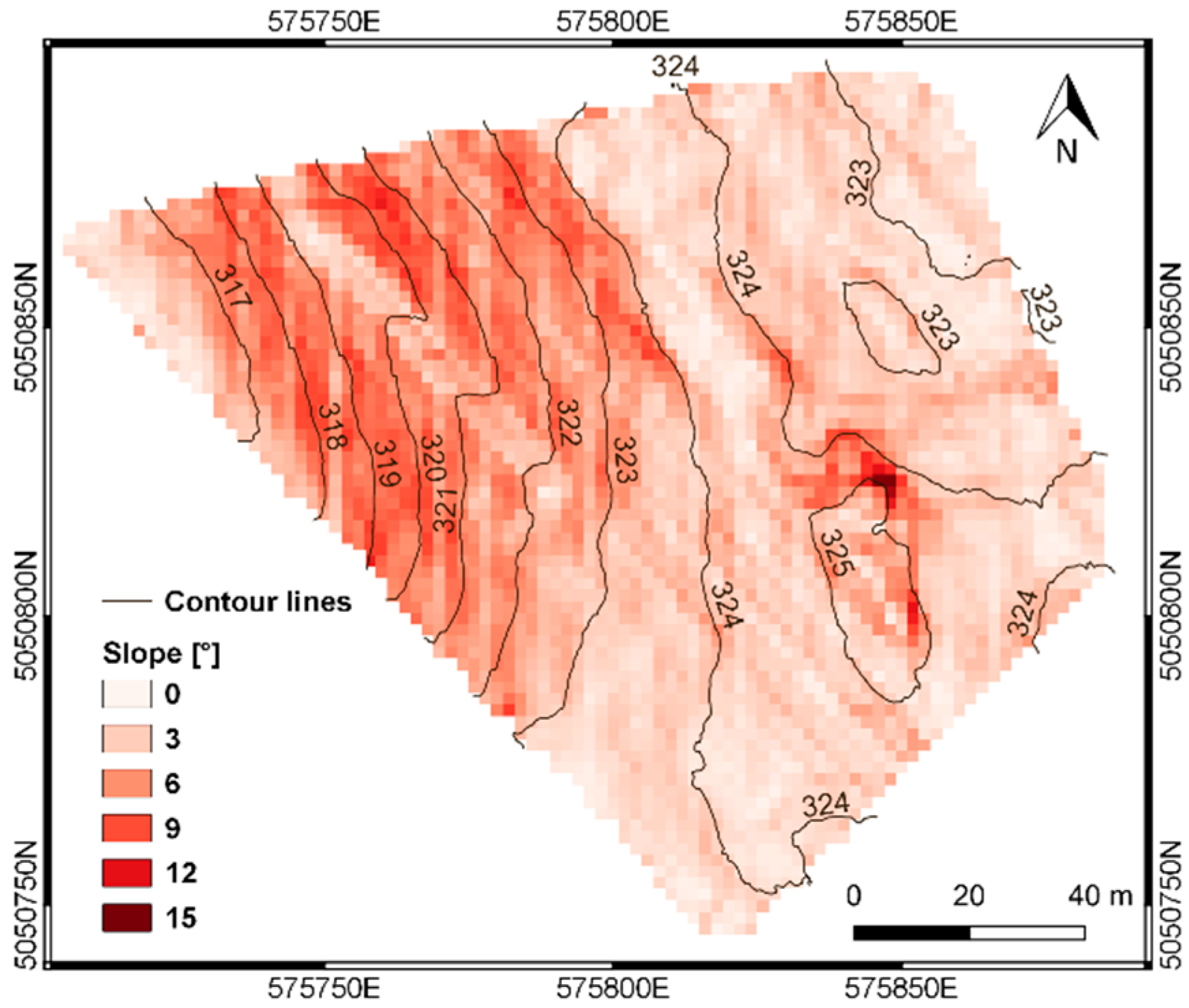
Figure 7.
Slope map and contour lines derived from the DTM.
Figure 7.
Slope map and contour lines derived from the DTM.
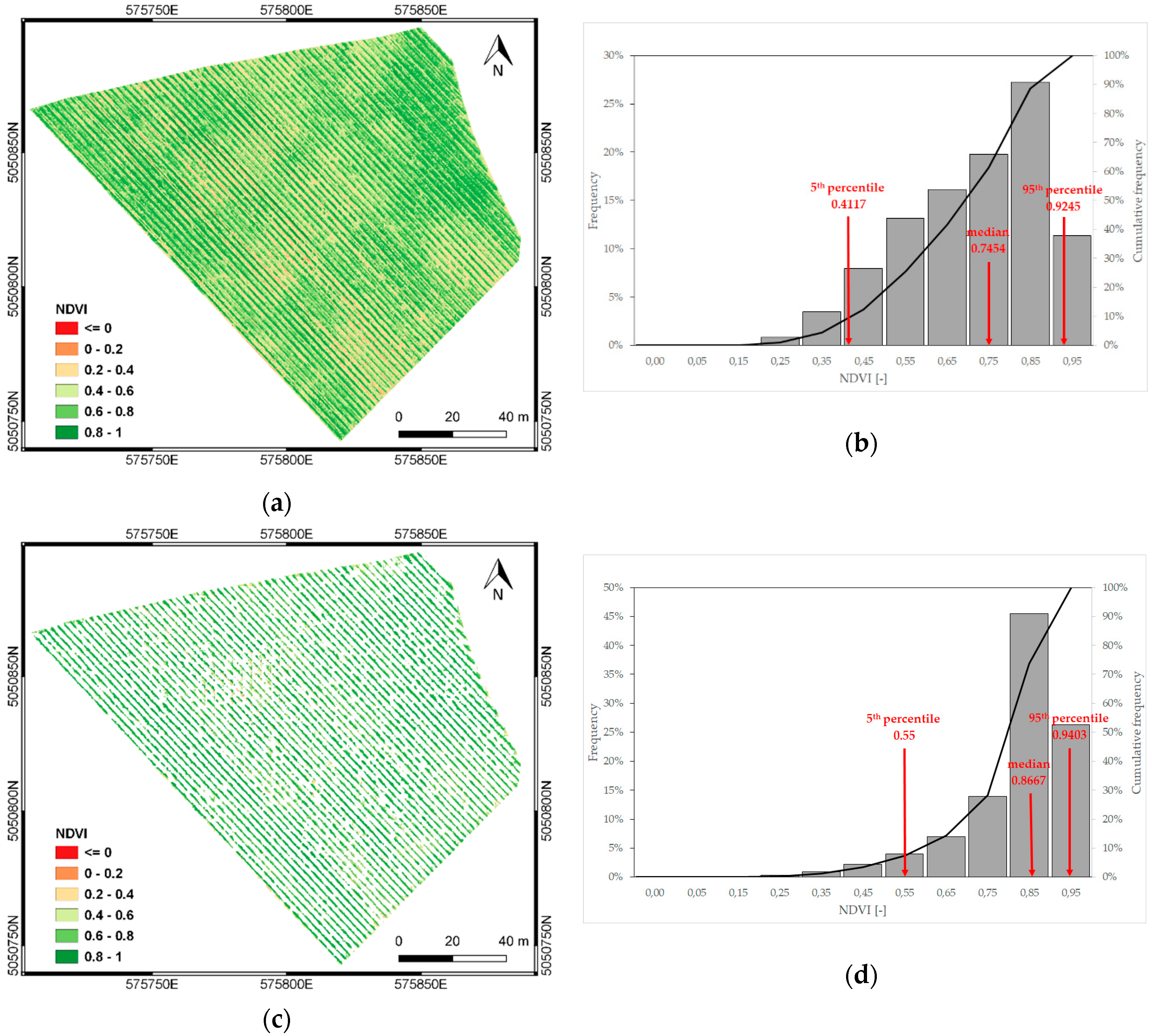
Figure 8.
NDVI map before (a) and after (c) soil masking, together with their respective frequency distribution (b,d).
Figure 8.
NDVI map before (a) and after (c) soil masking, together with their respective frequency distribution (b,d).
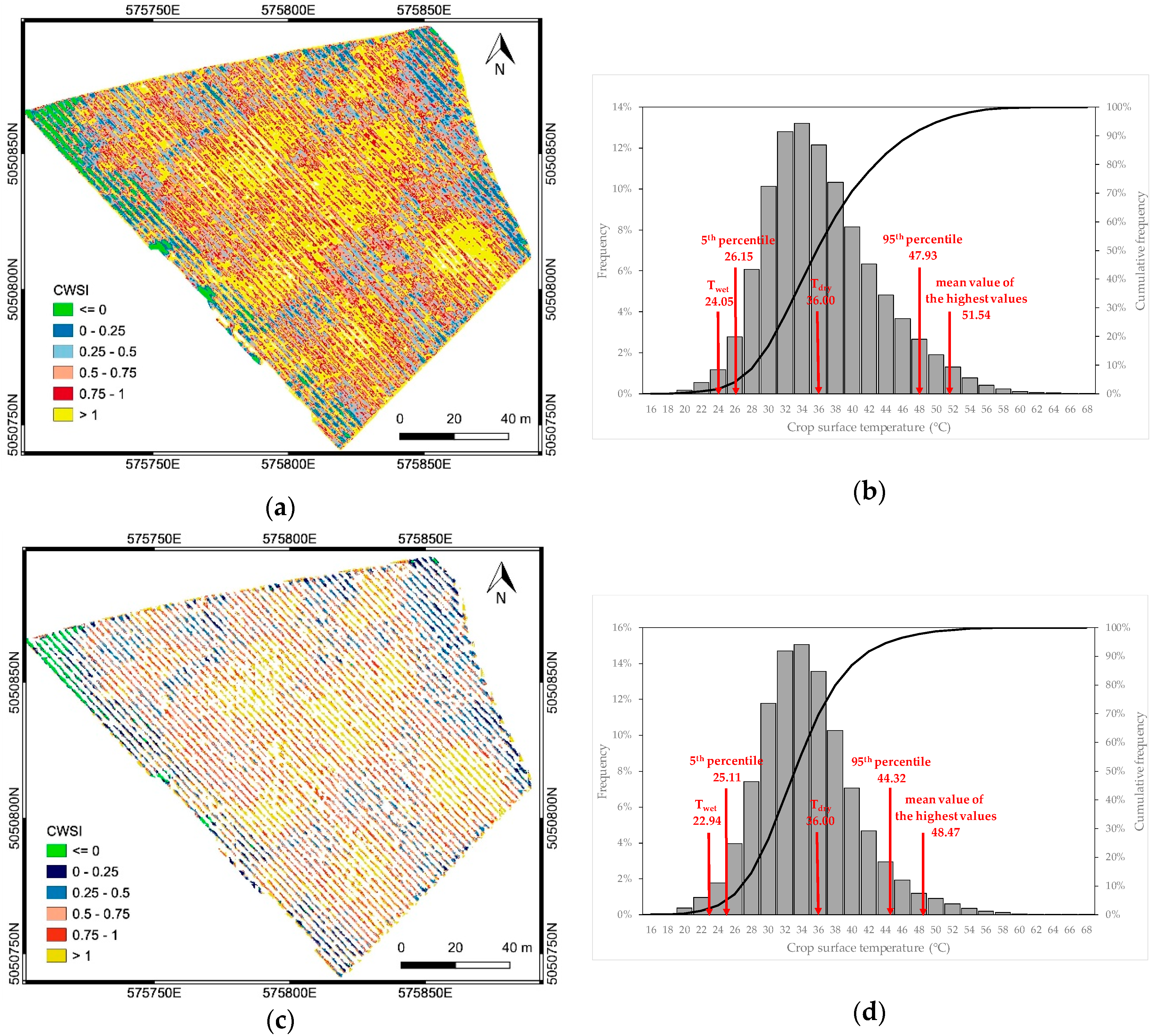
Figure 9.
CWSI map before (
a) and after (
c) soil masking. The frequency distribution of the crop surface temperatures, with the illustration of T
wet and T
dry values calculated according to the empirical approach described in
Section 3.1.3, is reported for each case (
b,
d).
Figure 9.
CWSI map before (
a) and after (
c) soil masking. The frequency distribution of the crop surface temperatures, with the illustration of T
wet and T
dry values calculated according to the empirical approach described in
Section 3.1.3, is reported for each case (
b,
d).
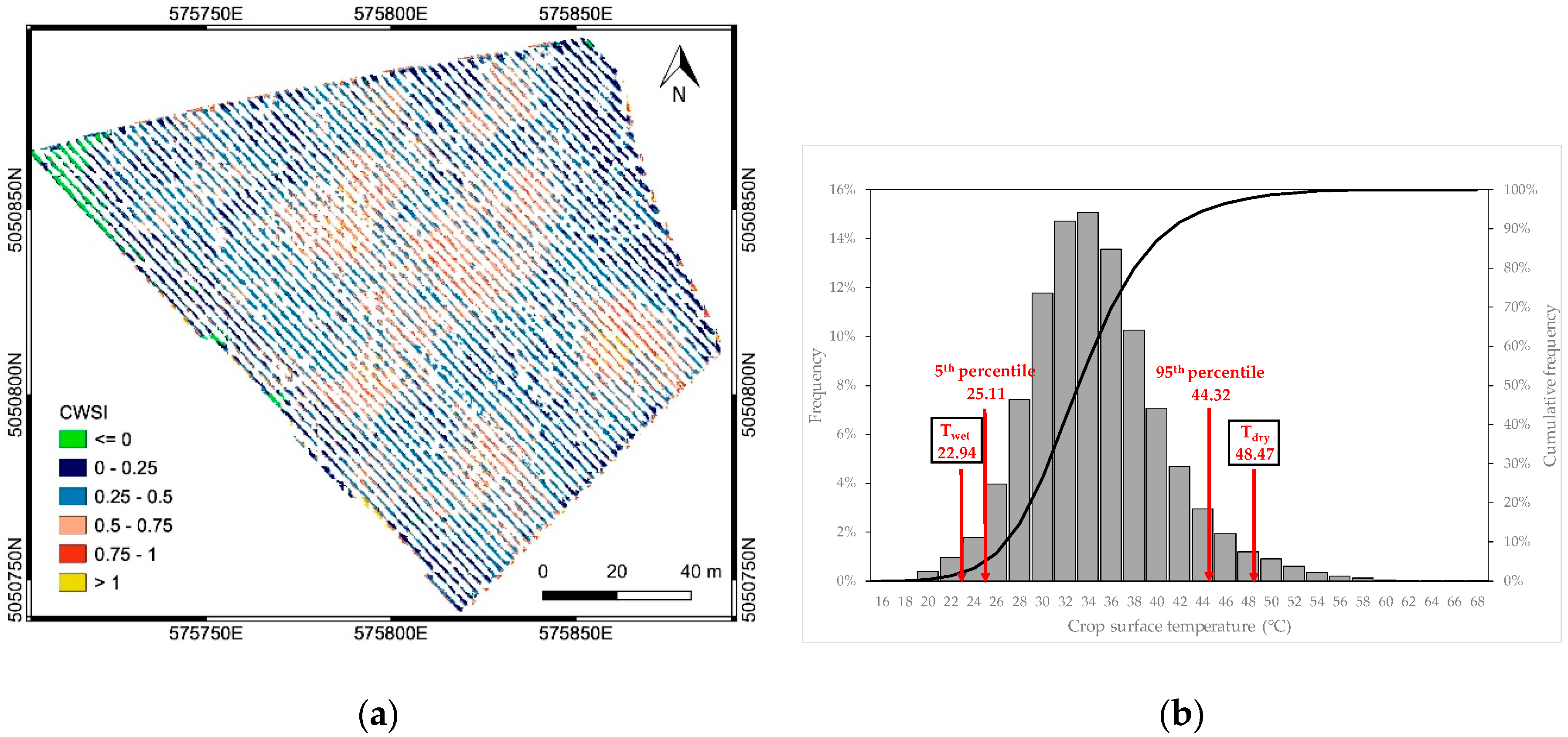
Figure 10.
CWSI map after soil masking (a), derived considering the Twet and Tdry values calculated as the mean of the coolest 5% and the hottest 5% vegetated pixels in the crop surface TIR orthomosaic, respectively. The frequency distribution of the crop surface temperatures is also reported (b).
Figure 10.
CWSI map after soil masking (a), derived considering the Twet and Tdry values calculated as the mean of the coolest 5% and the hottest 5% vegetated pixels in the crop surface TIR orthomosaic, respectively. The frequency distribution of the crop surface temperatures is also reported (b).
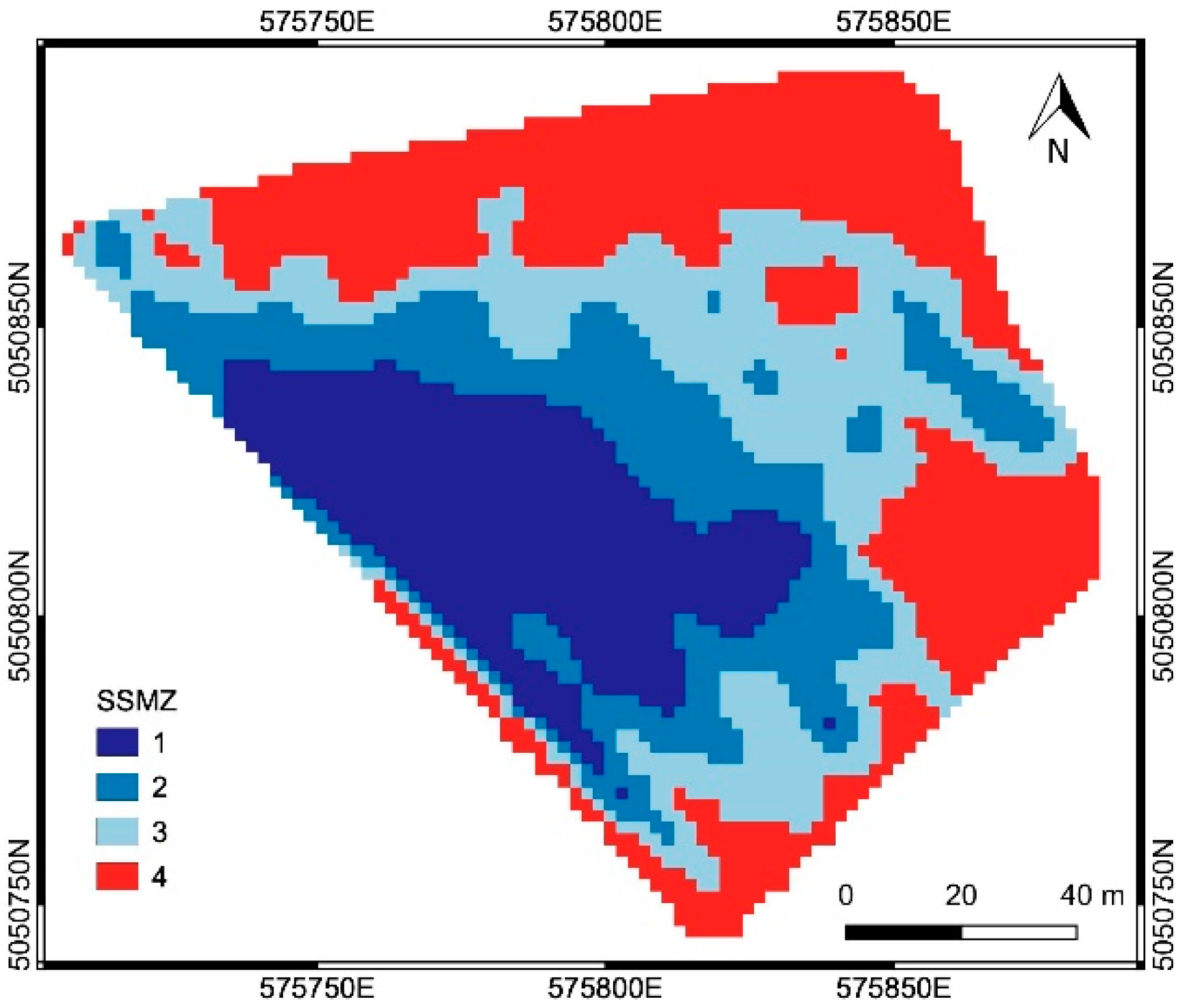
Figure 11.
The SSMZ map obtained from the EC maps relative to frequencies 15 kHz and 10 kHz. SSMZ from 1 to 4 corresponds to decreasing EC values; in particular, SSMZ 4 corresponds to negative EC values, due to gravelly soils.
Figure 11.
The SSMZ map obtained from the EC maps relative to frequencies 15 kHz and 10 kHz. SSMZ from 1 to 4 corresponds to decreasing EC values; in particular, SSMZ 4 corresponds to negative EC values, due to gravelly soils.
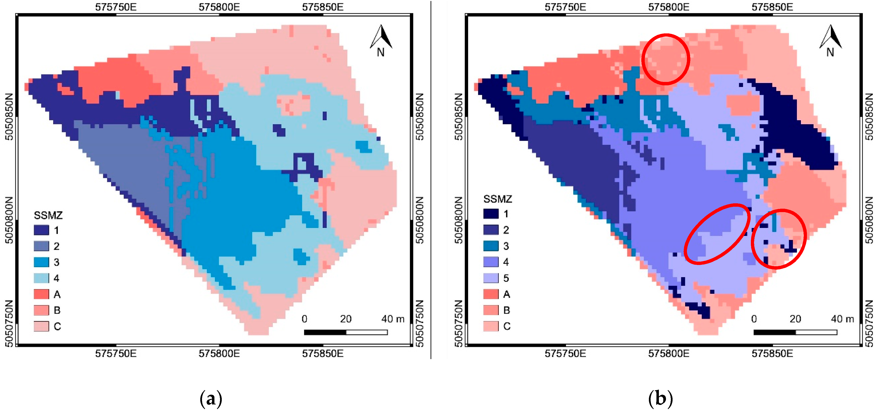
Figure 12.
The SSMZ map obtained from: (a) EC, elevation and slope maps; (b) EC, elevation, slope and NDVI.
Figure 12.
The SSMZ map obtained from: (a) EC, elevation and slope maps; (b) EC, elevation, slope and NDVI.
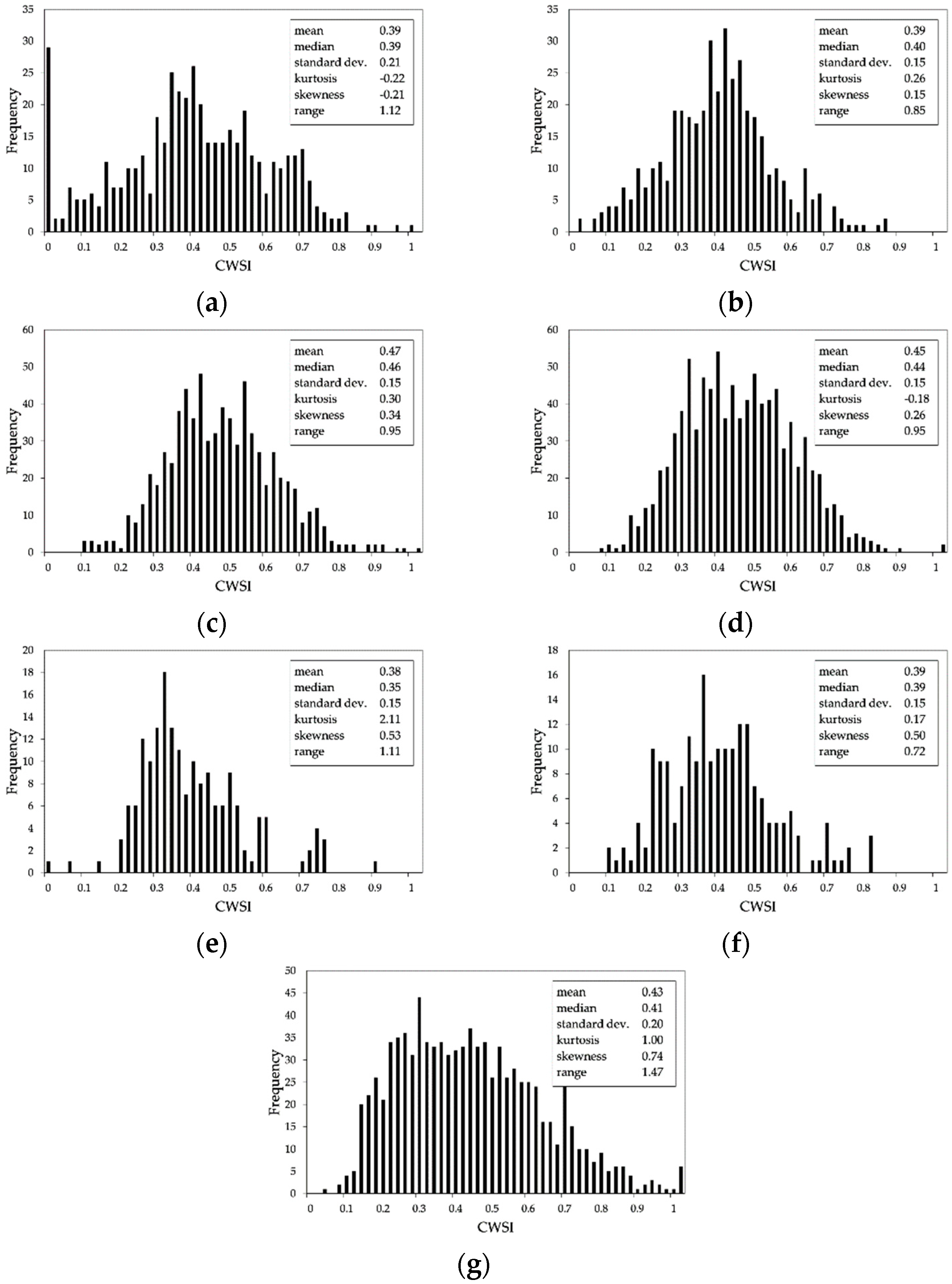
Figure 13.
Distribution of the CWSI values within each SSMZ shown in
Figure 12a: (
a) SSMZ 1; (
b) SSMZ 2; (
c) SSMZ 3; (
d) SSMZ 4; (
e) SSMZ A; (
f) SSMZ B; (
g) SSMZ C.
Figure 13.
Distribution of the CWSI values within each SSMZ shown in
Figure 12a: (
a) SSMZ 1; (
b) SSMZ 2; (
c) SSMZ 3; (
d) SSMZ 4; (
e) SSMZ A; (
f) SSMZ B; (
g) SSMZ C.
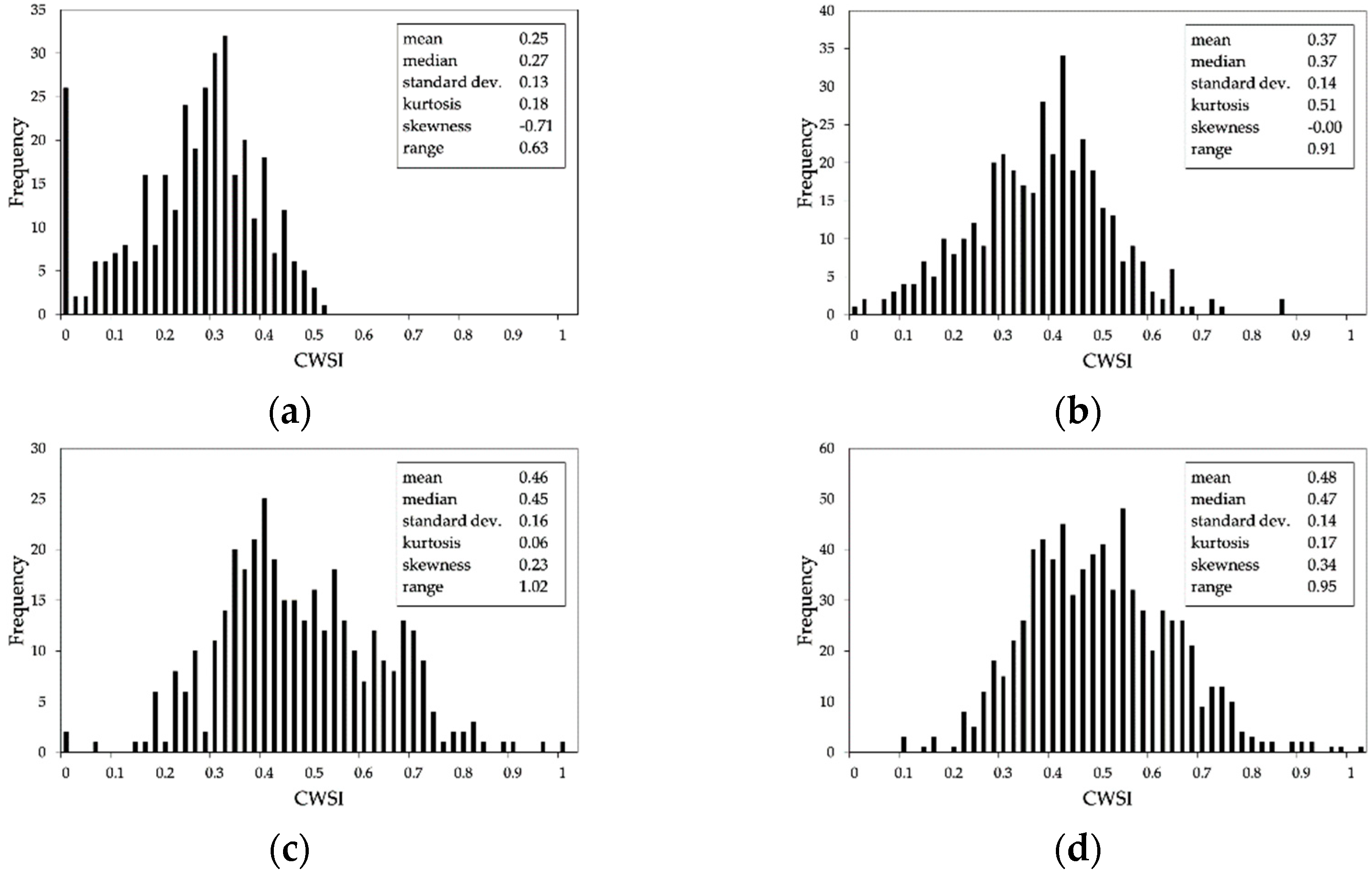
Figure 14.
Distribution of the CWSI values within each SSMZ shown in
Figure 12a: (
a) SSMZ 1; (
b) SSMZ 2; (
c) SSMZ 3; (
d) SSMZ 4; (
e) SSMZ 5; (
f) SSMZ A; (
g) SSMZ B; (
h) SSMZ C.
Figure 14.
Distribution of the CWSI values within each SSMZ shown in
Figure 12a: (
a) SSMZ 1; (
b) SSMZ 2; (
c) SSMZ 3; (
d) SSMZ 4; (
e) SSMZ 5; (
f) SSMZ A; (
g) SSMZ B; (
h) SSMZ C.
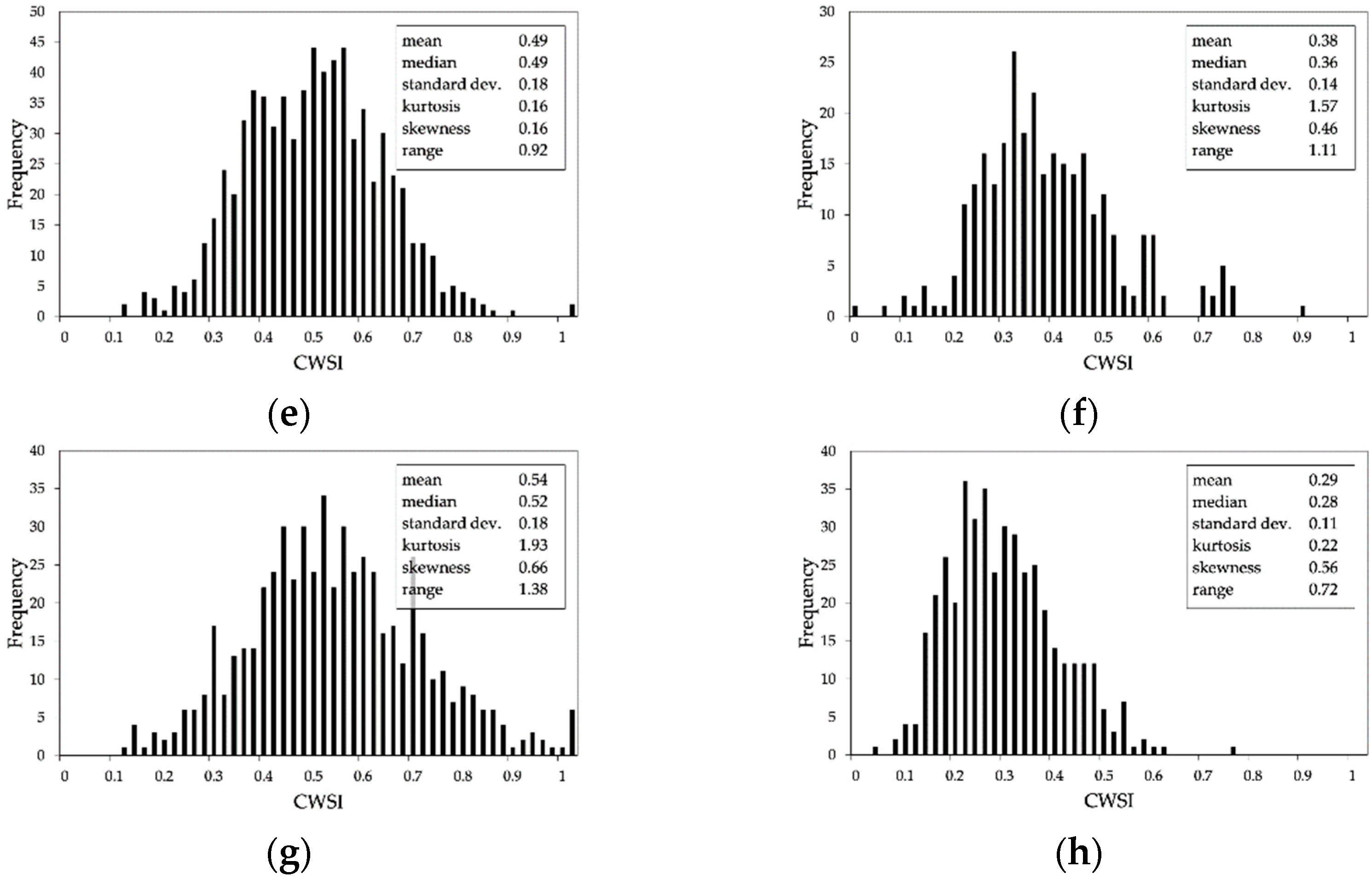
Figure 15.
Results of the PCA applied in the area ‘a’: spatial distribution of PCa1 (a), PCa2 (b) and PCa3 (c).
Figure 15.
Results of the PCA applied in the area ‘a’: spatial distribution of PCa1 (a), PCa2 (b) and PCa3 (c).
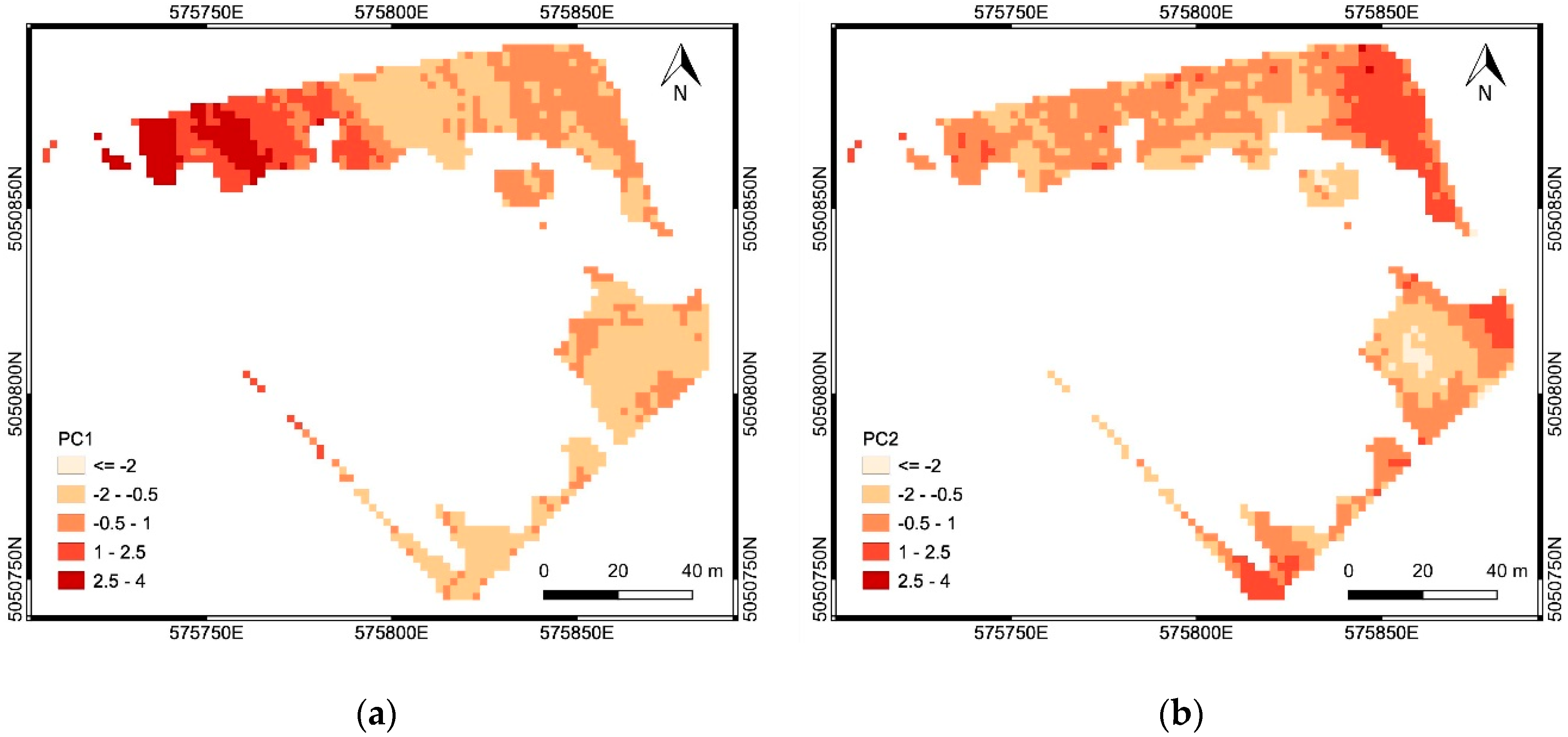
Figure 16.
Results of the PCA applied in the area ‘b’: spatial distribution of PCb1 (a), PCb2 (b).
Figure 16.
Results of the PCA applied in the area ‘b’: spatial distribution of PCb1 (a), PCb2 (b).
Table 1.
Technical specifications of the three cameras used for the vegetation survey.
Table 1.
Technical specifications of the three cameras used for the vegetation survey.
| | Survey 2 | SJ4000 | OPTRIS PI400 |
|---|
| Acquisition | VIS | NIR | TIR |
| Focal length (mm) | 4.35 | 4.35 | 8 |
| Sensor size (mm) | 4.86 × 3.64 | 4.86 × 3.64 | 9.55 × 7.2 |
| Sensor size (px) | 4032 × 3024 | 4032 × 3024 | 382 × 288 |
| Pixel size (μm) | 1.2 | 1.2 | 25 |
| Field of View (FOV) | 82° | 82° | 62° × 49° |
| Output format | JPEG image | JPEG image | RAVI video |
| Weight (g) | 64 | 64 | 380 |
Table 2.
Pearson’s correlation coefficients among the variables used to delineate SSMZ, estimated considering the grid nodes with valid EMI measurements (area ‘a’).
Table 2.
Pearson’s correlation coefficients among the variables used to delineate SSMZ, estimated considering the grid nodes with valid EMI measurements (area ‘a’).
| | EC-15 kHz | EC-10 kHz | DTM | Slope | NDVI |
|---|
| EC-15 kHz | 1 | 0.93 *** | −0.20 *** | 0.23 *** | −0.22 *** |
| EC-10 kHz | | 1 | −0.29 *** | 0.26 *** | −0.21 *** |
| DTM | | | 1 | −0.40 *** | −0.19 *** |
| Slope | | | | 1 | −0.07 ** |
| NDVI | | | | | 1 |
Table 3.
Pearson’s correlation coefficients among the variables used to delineate SSMZ, estimated considering the grid nodes with not valid EMI measurements (area ‘b’).
Table 3.
Pearson’s correlation coefficients among the variables used to delineate SSMZ, estimated considering the grid nodes with not valid EMI measurements (area ‘b’).
| | EC-15 kHz | EC-10 kHz | DTM | Slope | NDVI |
|---|
| EC-15 kHz | - | - | - | - | - |
| EC-10 kHz | | - | - | - | - |
| DTM | | | 1 | −0.40 *** | −0.12 ** |
| Slope | | | | 1 | −0.08 * |
| NDVI | | | | | 1 |
Table 4.
Moran Index among the variables used to delineate SSMZ, estimated (using GeoDa software, by Luc Anselin) considering the grid nodes with valid EMI measurements (area ‘a’).
Table 4.
Moran Index among the variables used to delineate SSMZ, estimated (using GeoDa software, by Luc Anselin) considering the grid nodes with valid EMI measurements (area ‘a’).
| | EC-15 kHz | EC-10 kHz | DTM | Slope | NDVI |
|---|
| EC-15 kHz | 0.82 ** | 0.79 ** | −0.20 ** | 0.23 ** | −0.24 ** |
| EC-10 kHz | | 0.81 ** | −0.28 ** | 0.27 ** | −0.22 ** |
| DTM | | | 0.99 ** | −0.40 ** | −0.19 ** |
| Slope | | | | 0.63 ** | −0.07 ** |
| NDVI | | | | | 0.76 ** |
Table 5.
Moran Index among the variables used to delineate SSMZ, estimated (using GeoDa software, by Luc Anselin) considering the grid nodes with not valid EMI measurements (area ‘b’).
Table 5.
Moran Index among the variables used to delineate SSMZ, estimated (using GeoDa software, by Luc Anselin) considering the grid nodes with not valid EMI measurements (area ‘b’).
| | EC-15 kHz | EC-10 kHz | DTM | Slope | NDVI |
|---|
| EC-15 kHz | - | - | - | - | - |
| EC-10 kHz | | - | - | - | - |
| DTM | | | 0.96 ** | −0.59 ** | −0.15 ** |
| Slope | | | | 0.69 ** | −0.09 ** |
| NDVI | | | | | 0.66 ** |
Table 6.
Results of PCA applied in the area ‘a’: variance of the principal components considered in CA and correlation coefficients with the variables used to delineate SSMZ.
Table 6.
Results of PCA applied in the area ‘a’: variance of the principal components considered in CA and correlation coefficients with the variables used to delineate SSMZ.
| | Variance | Cumulative Variance | EC-15 kHz | EC-10 kHz | DTM | Slope | NDVI |
|---|
| PCa1 | 2.26 | 45% | 0.90 | 0.93 | −0.48 | 0.52 | −0.27 |
| PCa2 | 1.29 | 71% | 0.25 | 0.18 | 0.72 | −0.45 | −0.69 |
| PCa3 | 0.87 | 88% | 0.28 | 0.26 | 0.03 | −0.61 | 0.59 |
Table 7.
Results of PCA applied in the area ‘b’: variance of the principal components considered in CA and correlation coefficients with the variables used to delineate SSMZ.
Table 7.
Results of PCA applied in the area ‘b’: variance of the principal components considered in CA and correlation coefficients with the variables used to delineate SSMZ.
| | Variance | Cumulative Variance | DTM | Slope | NDVI |
|---|
| PCb1 | 1.56 | 52% | −0.89 | 0.88 | 0.06 |
| PCb2 | 1.03 | 87% | −0.14 | −0.20 | 0.99 |
Table 8.
Correlation between CWSI and variables DTM, Slope and NDVI.
Table 8.
Correlation between CWSI and variables DTM, Slope and NDVI.
| | DTM | Slope | NDVI |
|---|
| Pearson’s coefficient | 0.29 *** | 0.02 * | −0.71 *** |
| Moran Index | 0.29 ** | 0.02 ** | −0.52 ** |


