By placing the UPFs at the network edge not only the network response time but also the bandwidth consumption can be significantly reduced. However, placing a UPF in every available EN results in a rise of costs and UPF relocations. Therefore, the main objective of the UPF placement stages is to determine the optimal number of UPFs and their location in the given EN infrastructure, so that 5G services requirements can be satisfied while costs are minimized. Please note that, unlike the ENPP, where the access nodes can be simplified as TGs, the UPFs placement is strongly dependant on the behaviour of their underlying end-users (e.g., service demand and mobility patterns).
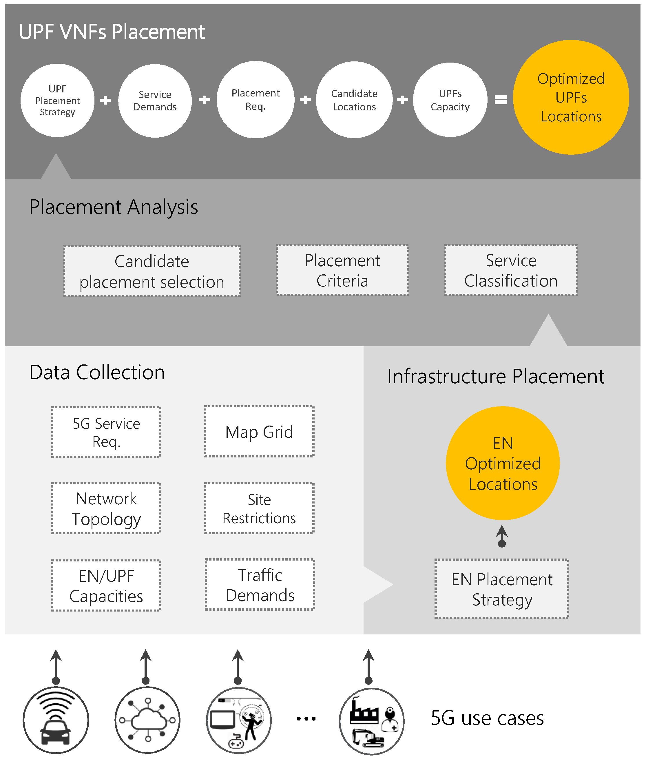
Taking into account the service classification,
placement criteria such as optimization objective and placement considerations are determined within the namesake module. For instance, the required number of backup UPFs for each service category is calculated according to its reliability level. The last module is responsible for selecting the candidate locations (i.e., ENs) for the UPF placement by taking into account available resources within the underlying infrastructure as well as the UPF maximum capacity and latency requirements of the service category. As a result, we obtain a set of UPF candidate locations for each access node (
) and a set of near access node for each candidate (
). To determine
and
, clustering techniques, i.e., Fuzzy C-means (FCM), are used. This method has been widely used in the area of allocation by various researchers [
28,
29]. Namely, FCM is used to determine the membership preferences between access nodes-candidate and candidate-access nodes.
4.2.1. Optimal UPF Placement
The OUP model aims at reducing deployment costs by minimizing the number of UPFs. Additionally, it also deals with the operational costs related to UPF relocations. However, not all users have the same mobility patterns, being many of them static sensors or indoor that produce zero relocations. Because of this, the proposed model allows distinguishing the optimization objective by taking into account whether the UPFs to be placed will serve users with mobility characteristics (m = 1) or not (m = 0). The OUP model can be formulated as follows:
Expressions (2a) and (2b) represent UPF placement costs for services with and without mobility requirements, respectively. In (2a), the first term is associated with the cost of deploying a UPF at location c () while the second term is related to the UPF relocation cost (). Hence, this objective function aims at optimizing both the deployment and operational expenditures by taking into account not only the number of UPFs to be deployed but the frequency of handovers in the (R)AN as well. For UPFs mostly serving users with zero or low mobility, Expression (2b) is more appropriate. In this case, the UPF placement costs can be determined in terms of the number of UPFs and their location dependent costs. Thus, the distinction of the objective function in terms of mobility requirements simplifies the problem formulation considerably when their effects on UPF relocations can be diminished.
The constraints of the system are described from (3) to (14). Expression (3) ensures that only a main or backup UPF is placed at a specific candidate location, thus guaranteeing only one UPF type for a given service category. Thus, in case of a failure in the infrastructure hosting a main UPF, its backup UPF can be instantiated in a safe location. Moreover, constraints (4) and (5) indicate that an access node must be assigned only to a candidate location where there is a main or backup UPF in place.
The constraint (6) guarantees that the demands of an access node are served by only a main UPF at a given time. In addition, restriction (7) forces the assignment of the access nodes to at least the minimum number of backup UPFs (−1) necessary to satisfy the service reliability requirements. Thus, each access node will be assigned to a total of UPFs (i.e., one main UPF and −1 backup UPFs). Additionally, Inequalities (8) and (9) ensure that the capacity of the main and backup UPFs is not exceeded by the underlying service demand. The factor defines the maximum capacity to be occupied in the main UPFs by the access nodes to avoid slowing their performance.
The Expression (10) ensures that the access nodes cannot be assigned to a main or backup UPF if the latency requirement () is not satisfied. The between (R)AN nodes and UPFs is determined by taking into account their processing time () and the service latency requirement (), . The effects of packet transmission and queuing delays in the overall latency are considered negligible. Moreover, constraint (11) restricts the assignment of an access node to a specific main UPF if this UPF has been placed at its location. Otherwise, it can be assigned to a UPF in any other location (12). Additionally, constraint (13) is an extra restriction to take into consideration for UPF placement with mobility requirements, Expression (2a). It expresses the relationship between two access nodes and their assignment to a main UPF. Since the Expression (13) is non-linear, it must be replaced by the following inequalities: , , and . Constraint (14) indicates that , , , and are binary variables.
4.2.2. Near-Optimal UPF Placement
The OUP model for non-mobility considerations is a variant of two well known NP-hard problems, the Resilient Controller Placement Problem [
30,
31] and the Hierarchical Capacitated Facility Location Problems [
32,
33], whereas its form for mobility requirements can be seen as a combination of the previous problems and the Location Area Planning problem [
5,
34] which is also NP-hard. Therefore, the OUP model, in either variant, is NP-hard. Hence, the OUP approach is not feasible for ultra-dense networking scenarios where the number of access nodes and candidate locations is quite large. In these scenarios, the number of possible combinations is extremely high and finding the optimal solution for the UPFPP may require excessive computation time and resources or lead to impractical solutions. To deal with this limitation, the NOUP algorithm has been developed. The pseudocode of the NOUP solution is shown in Algorithm 1.
| Algorithm 1: NOUP |
Input: , , , , , Access node demands (), , m,
Output: Set of total UPFs (), Set of UPFs service areas (), Set of unassigned access nodes ()
![Sensors 19 03975 i001]() |
The NOUP algorithm aims at finding the best locations and number of UPFs to serve a given set of access nodes at different resilience levels. The levels of UPFs are placed according to their role, starting with the main level and ending with the last level of backup. For each level, all the available candidates are evaluated and the best ones are selected. This approach guarantees that the best locations are selected and that these locations belong to UPFs with a higher role. Executing this algorithm outputs the location of the UPFs (), their service area () and the unassigned access nodes (), in case there are any.
The NOUP starts by initializing the output variables (line: 1). Afterwards, it proceeds to determine the UPF placement for the required levels (lines: 2–29). The first step when placing a level of UPF is to create the empty sets for the output variables in the corresponding level (i.e., , and ) (line: 3). Next, the access nodes to be assigned to a level of UPFs are selected (line: 4). To determine the best location for the UPFs each available candidate is analyzed by establishing its potential service area (lines: 6–22). This kind of area is formed by the unassigned access nodes near the candidate () that satisfy the latency requirement (lines: 7–8).
At this point, Algorithm 2 is executed, which is in charge of setting the UPF service area. Its first step is to ensure that restriction (11) of the problem formulation is satisfied (lines: 1–3). To achieve this, the algorithm checks whether the candidate is a main UPF co-located with an access node (line: 1). If this is the case, the (R)AN node is assigned to the service area and the UPF available capacity (), the unassigned access nodes near the candidate () and the UPF service area () are updated (lines: 2–3). Afterwards, the unassigned (R)AN nodes near the candidate () are sorted by their proximity to the candidate (line: 4) and an assignment process takes place (lines: 5–21). This process is repeated while the UPF candidate has available capacity and there are unassigned access nodes near it.
| Algorithm 2: FormingServiceArea |
![Sensors 19 03975 i002]() |
For the assignment, those access nodes that have the selected as unique candidate, known as critic access nodes (), are prioritized (lines: 7–8). If there are no critic access nodes the selection of an access node for its assignment to the candidate is made according to the UPF type and mobility requirements (lines: 9–13). Namely, if the service area belongs to a main UPF with mobility requirements (m = 1), the unassigned access node with the highest frequency of handover, with respect to the access nodes in the UPF service area, is selected (lines: 10–11). Otherwise, the chosen access node is the closest one to the candidate (lines: 10–13).
Once an access node is selected, it is necessary to check that it can be served by the UPF (line: 14). If the UPF has enough available capacity to serve the selected access node, the next step is to verify that no access node is affected by the assignment (line: 15). An assignment may affect other access nodes when their corresponding main UPF cannot be placed without violating constraint (11). If a critic access node cannot be served by the available capacity in the candidate, an error indicator is activated and Algorithm 2 is interrupted (lines 20). Otherwise, the set is updated by removing the selected access node (line: 21), regardless of whether it was assigned or not.
After Algorithm 2 is executed, the next step in Algorithm 1 is to verify whether the candidate service area was successfully created. If the execution of Algorithm 2 was interrupted due to the existence of an unassigned critic access node, a sub-process to find a candidate for the critic access node is launched (line: 10). If a candidate is found the node is assigned and the sets of UPF locations (), UPF service areas (), unassigned (R)AN nodes (), candidate locations () and candidate near the access nodes are updated (lines: 11–13). Otherwise, the critic access node is added to the set of unassigned access nodes () (lines: 14–15). In both cases, the candidate evaluation process is interrupted and restarted (line: 16). If Algorithm 2 was successfully executed, the candidate service area is inspected. If the service area is not empty, the candidate is evaluated and added to a list of valid candidates () (lines: 18–20). The candidate evaluation is made by taking into account metrics such as utilization, worst delay and relocation avoidance for mobility considerations. If the candidate has no assigned access nodes, it is removed from the set of candidates (lines: 21–22).
Once all the candidates are analyzed, the valid candidate with the best service area is selected (lines: 23–25). The best candidate is the one that has more access nodes assigned and avoids the greatest number of UPF relocations if m = 1. Each time that the best candidate is chosen, the sets , , , and are updated (line: 25). In case no valid candidates, the remaining access nodes in are added to the set of unassigned access nodes (lines: 26–27) and further analysis is required. These access nodes could be assigned to a UPF by relaxing the latency requirement or by deploying additional infrastructure. Notice, that these approaches imply either QoS degradation or the incurrence of additional costs. The candidate evaluation process (lines: 5–25) is repeated while there are unassigned access nodes.
Algorithm 3 is executed (line: 28) after a level of UPFs is placed. Its main objective is to reduce the number of UPFs and the relocation occurrence if mobility requirements are considered. Hence, Algorithm 3 first step is to determine the overall available capacity () in the UPFs of the level (line: 1). This capacity is compared with the UPF maximum capacity (line: 2). If the overall available capacity is higher than the UPF maximum capacity, the number of UPFs could be reduced (by removing some of them). To delete the lowest utilized UPFs, they are sorted and analyzed in descending order according to their available capacity (line: 3). For each UPF at level , it is checked whether all its assigned access nodes can be served by other UPFs (lines: 5–12). If an access node can be reassigned to other UPF, this is indicated by marking the access node (lines: 7–8). If all the access nodes in a UPF service area can be served by other UPFs, they are reassigned and the UPF is deleted from the set of UPFs (lines: 9–11). As a result of this process, the set of UPFs at level , their service areas, the available candidates and the candidate locations for each access node are updated (line: 12).
| Algorithm 3: Reassignment |
![Sensors 19 03975 i003]() |
Moreover, for a level of main UPFs with mobility requirements, Algorithm 3 tries to reduce the occurrence of relocations (lines: 13–18). For each access node that has been assigned during this level, it searches for whether there is a better UPF (lines: 15). If a better UPF in terms of relocations avoidance is found, the access node is reassigned and the UPF service areas are updated (lines: 16–18). At the end of this algorithm, two additional steps can be included to ensure that each access node is assigned to its nearest UPF and to reduce the load imbalance.
Finally, in Algorithm 1, the output sets are updated and the level indicator is decremented (line: 29). Steps 2–29 are repeated while there are available candidates and levels of UPFs pending for placement.


