1. Introduction
Land cover provides basic geospatial information for applications in the fields of global environmental change, natural resources management, carbon and nitrogen cycle, and ecological monitoring [
1,
2,
3]. Because of the continuous earth surface scanning and the correspondingly long-term data archives, satellite remote sensing is proven as an effective way in mapping global land cover and measuring land cover dynamic change [
4]. Currently, national and international agencies have successfully created no less than ten global scale land cover datasets with spatial resolutions of 1 km, 500 m, 300 m, 30 m, and 12 m. These existing land cover datasets provide basic geographic information for studying climate, hydrology, environment, ecology, and urban regions [
5,
6,
7,
8]. Their accuracies are undoubtedly one of the most concerning issues for the potential users. Although data accuracy or uncertainty information is given at the same time as the land cover product releases [
9,
10], users in different application fields generally need to verify the accuracy before making a decision in using the land cover product [
11,
12].
Sampling inspection is a commonly used method for verifying the accuracy of land cover products. It provides reliable information on product quality and uncertainty [
13,
14]. Determining the sample size, as a key procedure in the sampling scheme, lays the foundation for the later stages of sample displacement and verification. A reasonably-estimated sample size is an effective way to avoid the phenomena of over-sampling or under-sampling [
15,
16]. In addition, the sample size also affects the number of investigators, and the cost and time of the field investigation. Therefore, the estimation of sample size is not only important theoretically, but also plays a guiding role in scientific research and field work investigation.
Currently, there are three major sample size estimation methods: empirical values, fixed-grid sampling, and calculation from a statistical model. The empirical values are the sample numbers required by researchers to test the accuracy of each category of classified satellite images. For example, Hay provided at least 50 empirical values for samples in each category initially [
17], although the sample size could be enlarged with an increase in spatial regions and/or the amount of categories involved in the image classification. Congalton provided 75–100 sample data for each category of classified image, which are common empirical values for testing classified images [
18]. Empirical sample sizes are simple and can achieve the goal of sample representation through spatial optimization in the process of sample placement. It is usually used to determine the sample size in remote sensing products, especially in an accuracy assessment of classified images. However, with the sprawl of spatial regions, the spatial heterogeneity can vary to a large extent around the entire region(s).
A fixed grid is another commonly used method for determining a sample size for performing an accuracy assessment. It divides the study area into regular grids with a certain size, for instance, 1 km or 10 km, and a sample from each grid is required [
19,
20]. Ridder used a 10 km × 10 km grid and randomly selected 9000 samples to assess the accuracy of a global forest dataset [
21]. Stehman designed a 5 km × 5 km grid, in which 500 grids were randomly selected by synthesizing information on global climate zones and population density [
22,
23]. Through designing a sample encryption algorithm, a dataset for the verification of global land cover products was generated. This dataset can be used to validate other 1 km or 500 m resolution land cover datasets. The fixed grid sampling method is easy to implement, but the determination of grid specifications relies more on expert knowledge.
A statistical model is widely used to calculate a sample size. This method is based on theories of traditional probability and statistics [
24,
25]. Tong calculates sample sizes from two scales, one on the level of map divisions, and the other on the level of map elements [
26]. By establishing probability distribution functions in each scale, the calculated sample size overcomes the problem of ‘too strict in map divisions and too wide in map elements’, which commonly exists in classical sampling schemes. Based on probability and statistics theory, Olofsson calculated a sample size for simple random sampling and stratified sampling methods respectively, using a statistical model [
27]. As compared with the empirical or fixed-grid method, the statistical model is based on theories of statistics and probability. However, the sample size obtained by this method relies on the expected classification accuracy and sampling error information of the products. One of the main problems is that the same remote sensing product in different test sites with different areas will obtain the same numbers of samples, indicating that the surface spatial characteristics, such as patch numbers, aggregation, and diversity, from different study sites, are not involved in the calculation of sample size.
Until now, the determination of a sample size has primarily relied on expert knowledge or conditional assumptions. This often makes it difficult to ensure the rationality of the sample size. Therefore, this study addresses how to determine a number of samples while considering surface spatial heterogeneity.
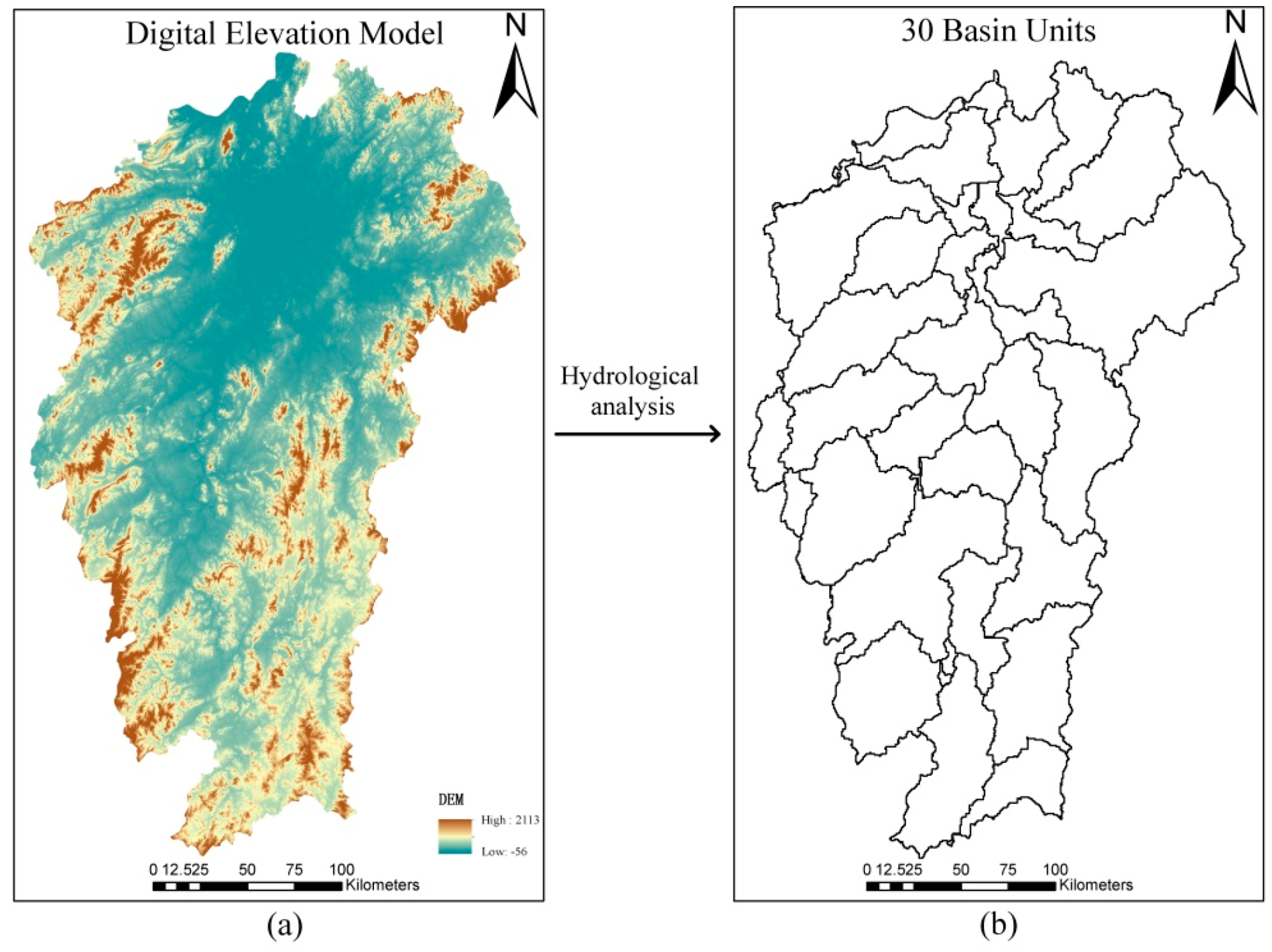
Statistical theory is the foundation for determining the sample size. This study derived a sample size estimation using a stratified sampling approach. Then, a multi-level linear sample size estimation model was developed by considering the scale effect and surface spatial heterogeneity, with emphasis on two aspects of these issues. First, a watershed unit with ecological and geographical significance was introduced in this study as the basic spatial unit for performing the accuracy assessment, avoiding the objectivity issues existing in current spatial units of pixels or polygons [
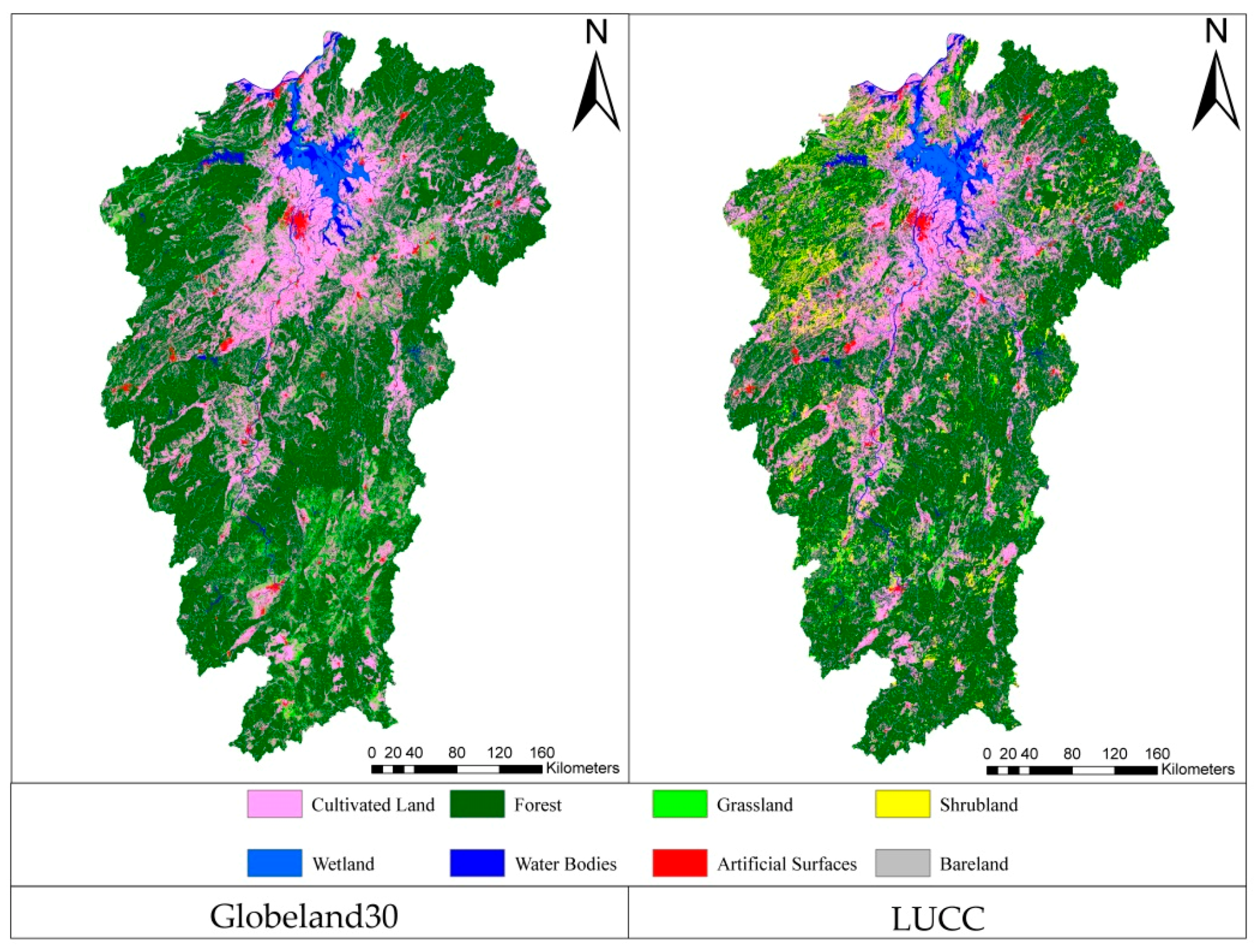
28]. Second, landscape indicators were employed to describe the surface heterogeneity and complexity. As the characteristics of the spatial heterogeneity would inevitably affect the sample size used for validating the land cover dataset, this study computed several major landscape indicators and assessed their impacts on the surface heterogeneity in watershed units, thereby reaching the goal of this study (to develop a reasonable model to estimate the sample size).
The remainder of the paper is organised as follows.
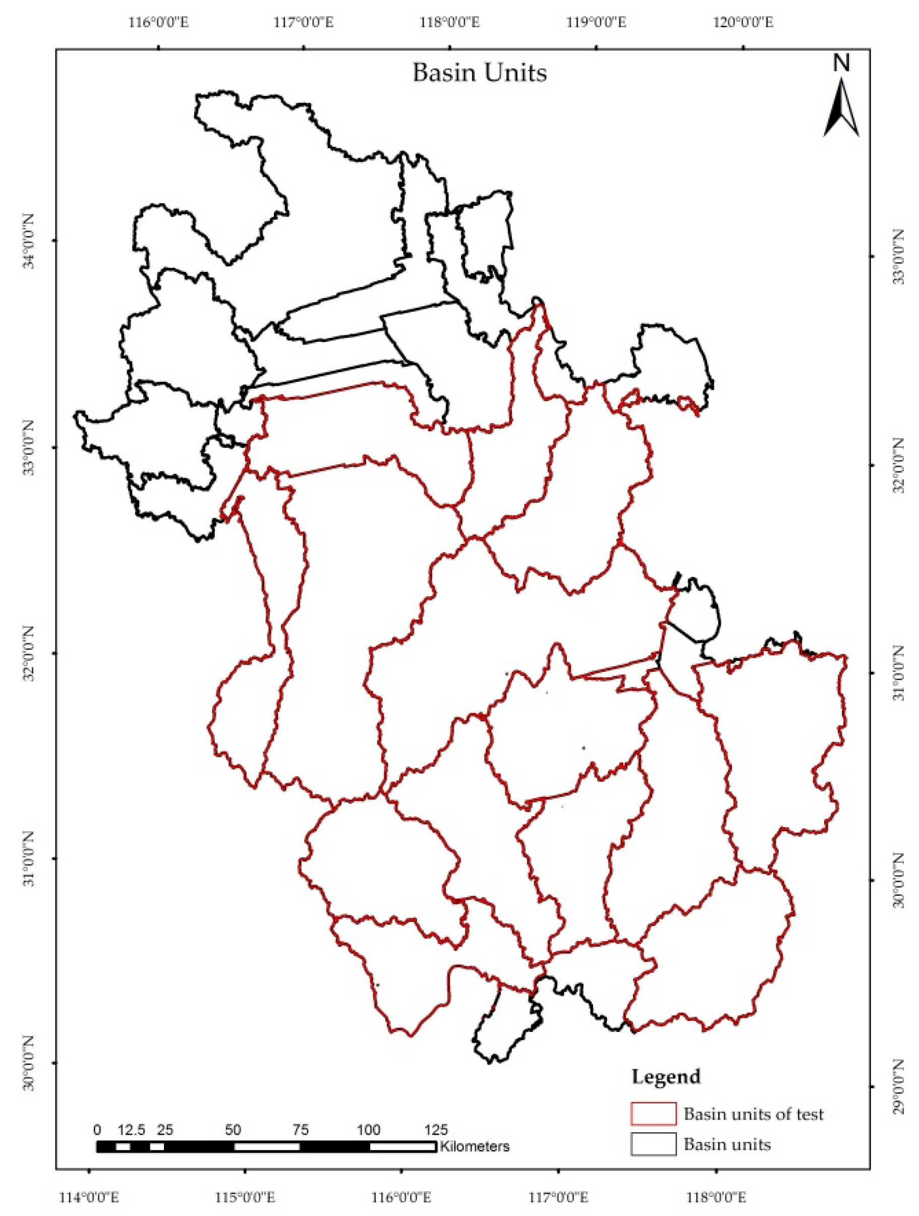
Section 2 introduces the study area, data sources, and data pre-processing methods.
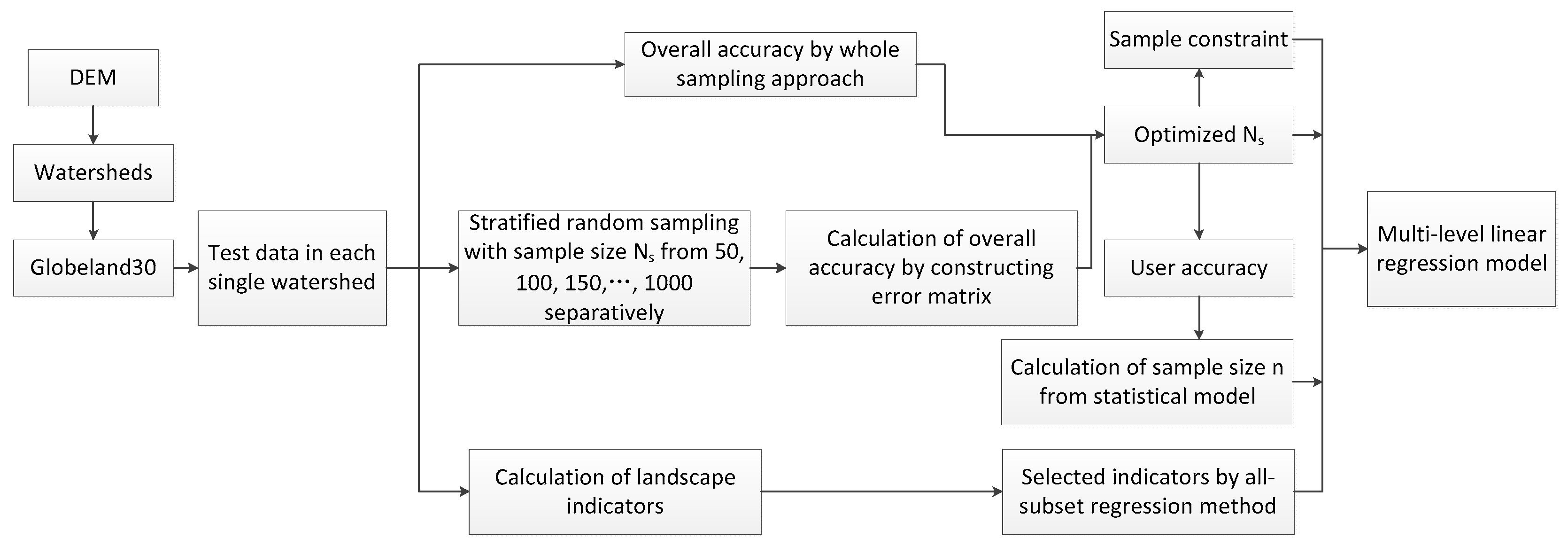
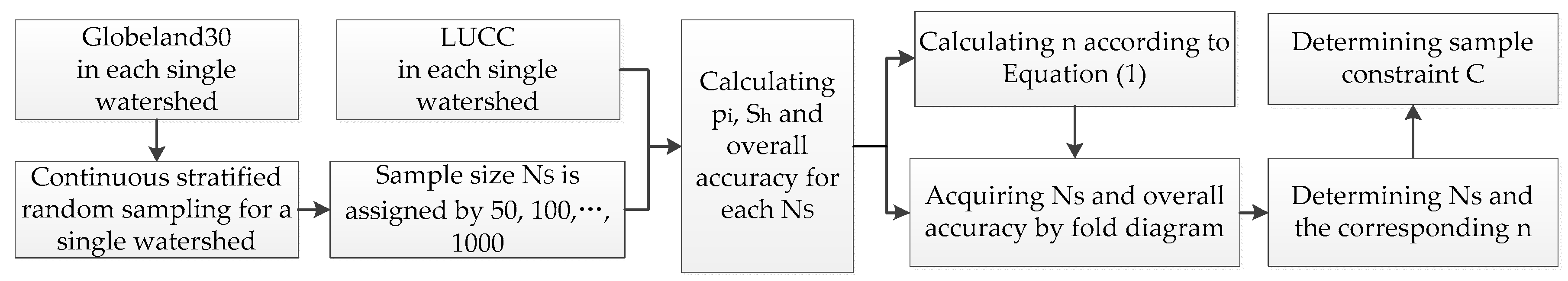
Section 3 describes the commonly used statistical model of sample size estimation, the selection of scale factor and landscape indicators, and the development of the multi-level linear regression model.
Section 4 presents results and an analysis of the developed model, and
Section 5 provides preliminary conclusions.
5. Conclusions
The accuracy of a dataset is often the first problem to be considered in scientific research and field applications. Sample size calculation is the first step in performing an accuracy assessment of land cover products from satellite imagery. On the basis of a statistical model for the estimation of sample size, this study establishes a multi-level linear model for estimation of sample size by considering the scale effect and spatial heterogeneity. A watershed unit was introduced to obtain a spatial analysis unit, to avoid subjectivity in the selection of assessment units. Landscape indices were selected to indicate the spatial heterogeneity of the region.
The multi-level linear sample size estimation model shows that:
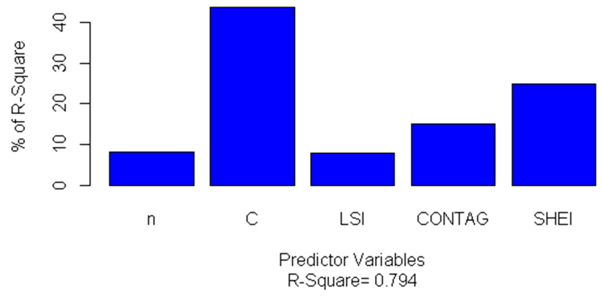
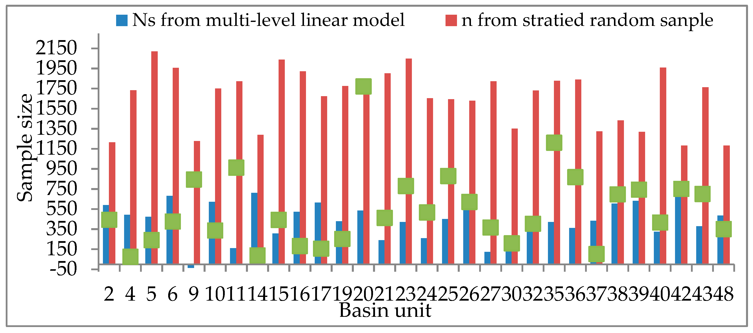
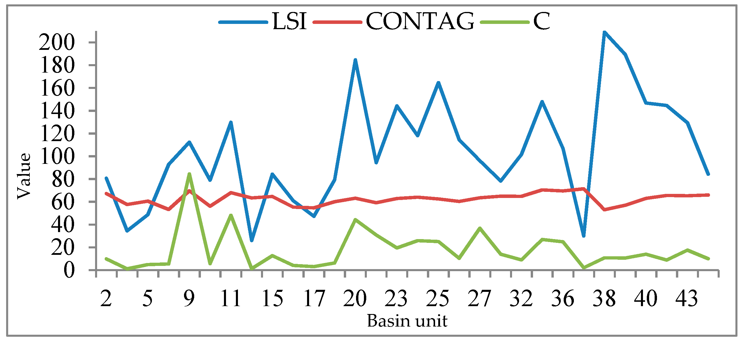
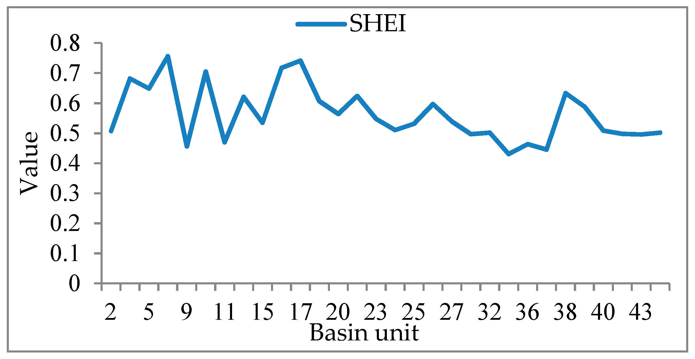
(1): All predictive variables can explain 79% of the variance of the sample size NS. The coefficients of the predictive variables of the model are significant, indicating that there is a strong relationship between the sample size NS and the independent variables. By comparing the sample size NS from the multi-level linear model with a sample size n based on probability and statistics theory, we see that the sample size of NS is much smaller than that of n. The smaller sample size can achieve the same performance as the statistical model and it contributes to the consideration of surface heterogeneity. The relative importance of the predicted variables in the model is calculated by using standardised regression coefficients and relative weights. The results show that the CONTAG and SHEI indicators (describing the diversity and dispersion of basin units, respectively) are relatively important, followed by LSI, sample constraint C, and sample size n, as calculated from probability sampling theory. According to the validation of the developed model, we can conclude that the smaller sample size from the developed estimation model can achieve the same performance as the statistical model while saving more time, cost, and energy in the accuracy assessment of land cover products.
(2): After performing three-fold cross-validation, the R2 value changes from 0.79 to 0.63. This means that the generalization of the sample size estimation model is still a problem, although the test of the model in the Anhui Province proved the validity of this estimation of sample size. Therefore, we need more work on the improvement and testing of the developed model for sample size estimation.
For a specific work on accuracy assessment, although the model established in this study cannot be directly applied, it is expected to provide an approach for the determination of sample size, by considering the study areas and the characteristics of the surface heterogeneity. In the future, we need to improve the developed model by applying this surface heterogeneity-concerned sample size estimation model to other study sites, aiming to assess the accuracy of a land cover dataset with as few samples as possible.


