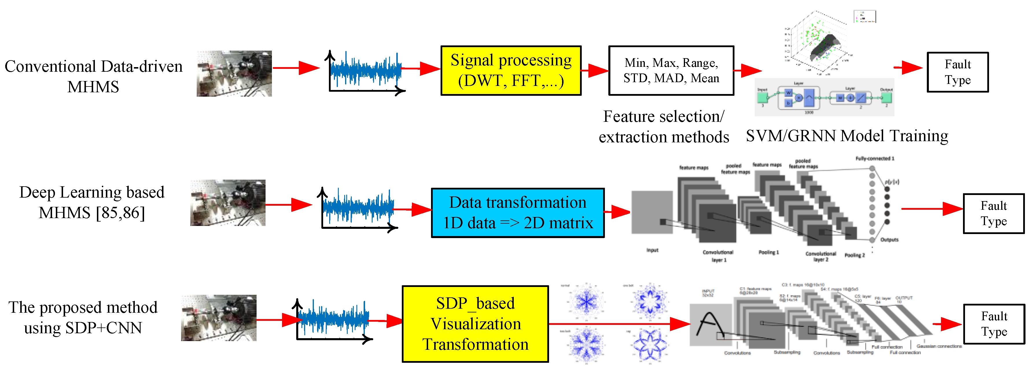
The main purpose of this project was to develop a method for the diagnosis of malfunction in the ball bearings of an electrical motor and to use vibration signals generated by bearing rotation, to determine the presence of abnormality. A malfunction simulation system was configured in the scheme to introduce malfunction, explanations of which are in the experimental-setup section. The frequency of ball-bearing vibration signals and the process under wavelet domain are explained in the analysis and process-of-vibration-signals section. A discussion of the formula for computing the feature is introduced in the motor-signal-features section. Machine learning, teaching, and classification by CNN, as well as visualization of the signals, are fully elucidated in the teaching-and-classification-of-CNN and machine-learning (ML) sections.
2.1. Experimental Setup
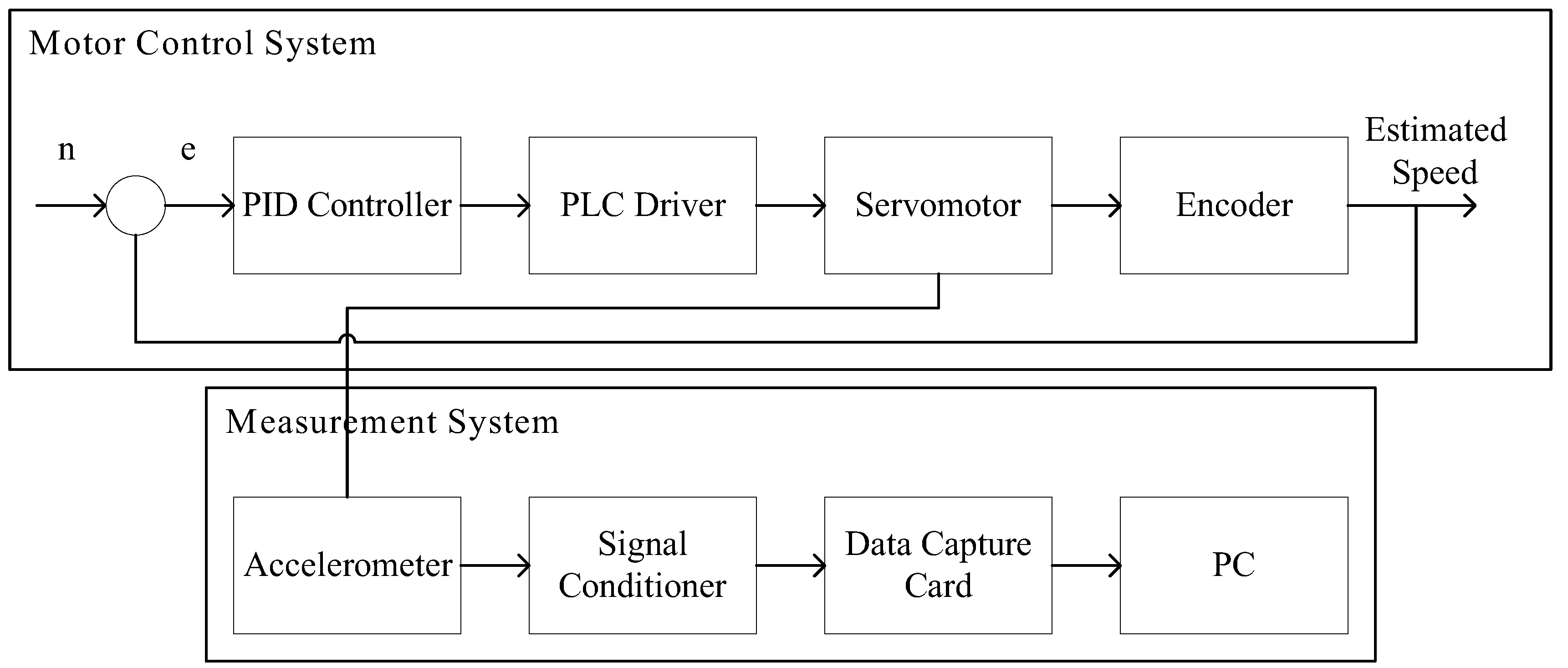
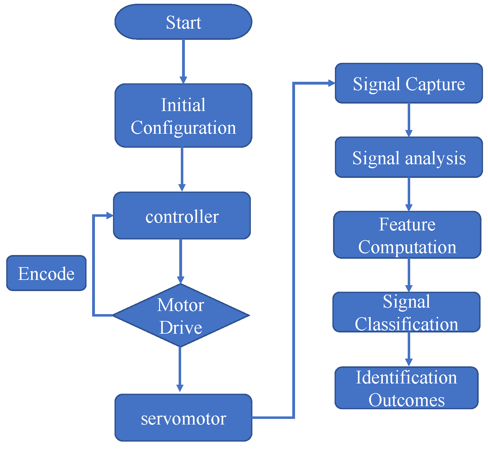
The major structure of this system includes a motor control system and measurement system. The motor control system manages to bridle a motor through a PC and BeckHoff controller and uses a PID controller algorithm. A set of human-machine interface (HMI) is built into the PC to monitor motor status in real time. As for the measurement system, it can capture the signals from the accelerometer through NI myRIO embedded system, as well as signal conditioner. Both the motor control system and measurement system are applied to the motor measurement platform developed in the lab, which is shown in
Figure 1; the related hardware specifications listed in
Table 1.
The BeckHoff controller is an embedded PC installable in DIN guide rails which includes a CX-series (CX5140) PC and an I/O module. This series features low power consumption and a fan-free design. It has one 4-core Intel® Atom™ CPU (1.91GHz) two independent Gigabit Ethernet ports, four USB2.0 ports, and one DVI-I port. The software included is the TwinCAT (Windows Control Automation Technology) system that was developed by BeckHoff and can interface with a PLC (Programmable Logic Controller) and NC/CNC. This PC is a fully functional controller. TwinCAT is compiled as a Run-Time system, which can run many programs, conduct diagnoses, and is fully configurable.
The drive module for the servomotor is an EL2111, which has an adequate capacity for the purpose. EtherCAT (Ethernet for Control Automation Technology) was used for communication and the client/server (C/S) model only needed a standard Ethernet card to connect to the host controller of the master terminal. The main application is automation, and a field-bus of an industrial control system (ICS) was used. The system has wide compatibility and is expandable. It is easy to operate and synchronizes very well. No specific hardware interface card was not needed, and connection was made using an Ethernet controller and a network port.
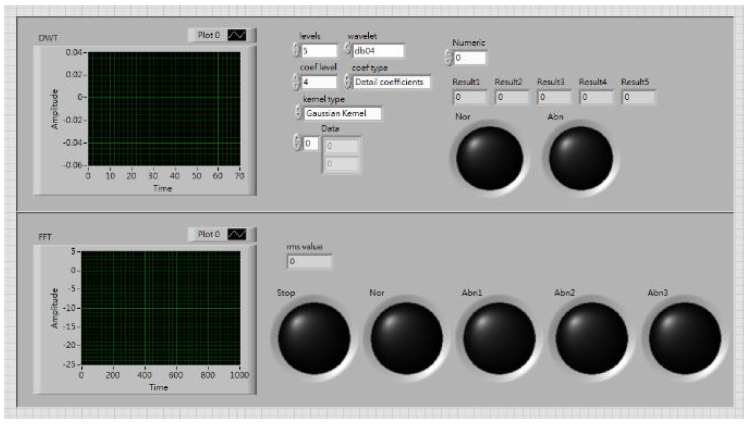
LabView captured the signals from the myRIO and transferred them to the PC terminal, for computation and classification through global variables. The graphical user interface (GUI) is shown in
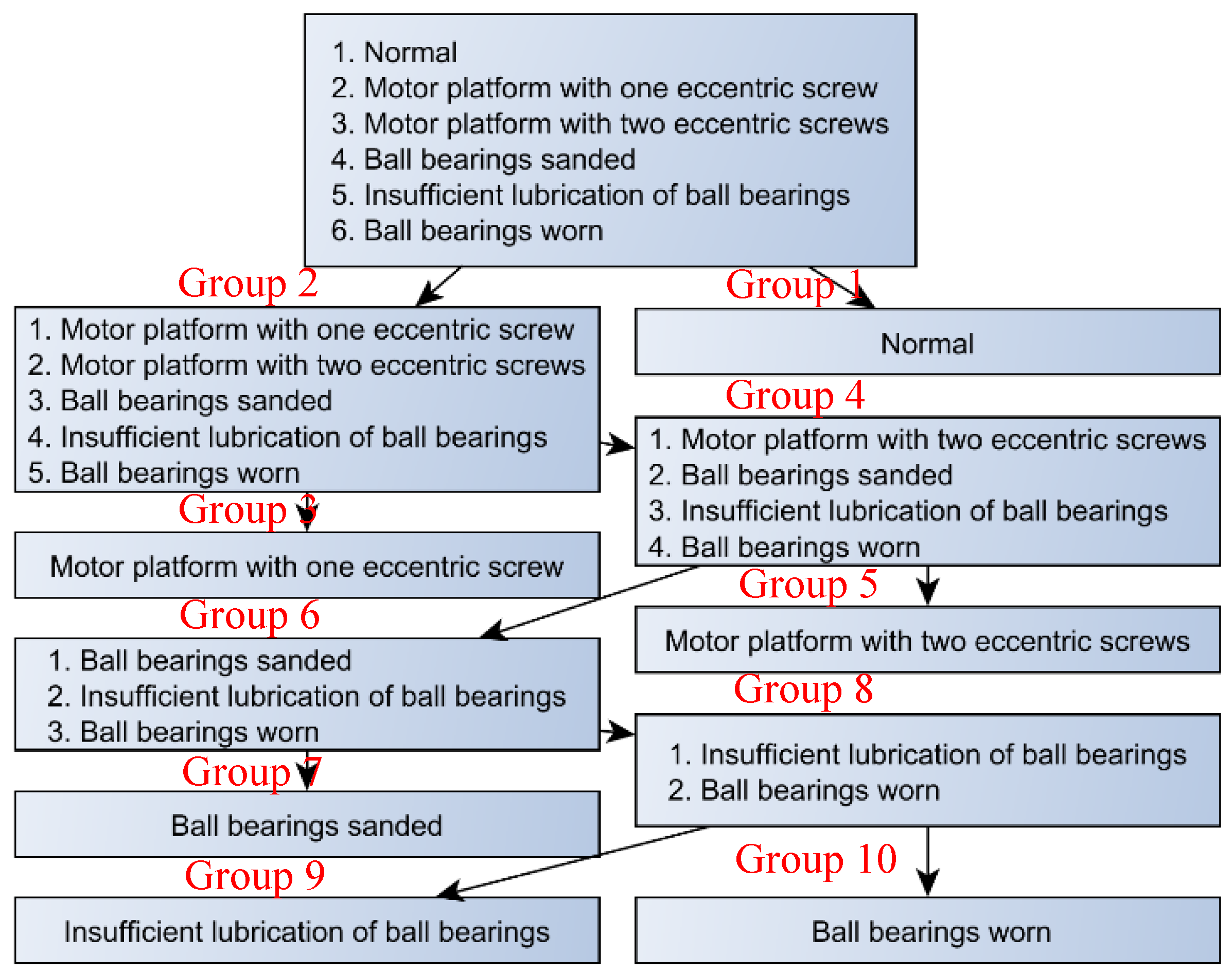
Figure 2. Six status conditions were used: (1) normal; (2) motor platform with one eccentric screw; (3) motor platform with two eccentric screws; (4) sanded ball bearings; (5) insufficient lubrication; and (6) worn ball bearings (see
Figure 3).
2.2. Analysis and Process of Vibration Signals of Ball Bearings
In this section, the principal analysis and processing of signals is introduced. As explained in the experimental-setup section, all the signals were transferred to the PC terminal, where the features were transformed either in the frequency domain or as discrete wavelets, before analysis. The results of the diagnoses, using the different classifiers, are shown in
Figure 4.
The vibration signals collected from various time domains and with different motor status are mixed with lots of noise from different frequency bands, and this presents a problem. To find useable features in the time domain, the signals need to be analyzed and treated before features can be selected for calculation. In this study, the vibration signals were first transformed in the frequency domain by FFT, a linear integral transform. It can transform the signals between time domain and frequency domain, and it can also decompose the time-domain signals into the superposition of sine waves from many different frequencies. The formula is shown as Equation (1):
where
is the input signal of continuous time,
is the angular frequency, and
is time. However, if the signals are represented by a form of discretion and periodicity in both the time domain and the frequency domain, it is a discrete Fourier transform (DFT). If the volume of data is large, the calculation of DFT can be enormous, and computation time will be long, where the computational complexity will be
. The fast Fourier transform (FFT) is a quick approach to the calculation of DFT. When dealing with general signals, the computation volume of FFT is much less than that of DFT, where computational complexity is
. FFT has excellent analytical performance for stationary signals where frequency does not change over time, but it cannot be used for time variation analysis of nonstationary signals. Locality does not exist, and it is only compatible with stable signals.
To provide a solution to this problem, Gabor proposed the short-time Fourier transform (STFT), which is a window function, and the formula is as in [
22]:
where
is the window function, and
is the translation parameter. The window function can split up the signals into many small time intervals, where the Fourier transform
can be done in a local time domain
, the position of the window function
is changed along with the translation parameter
, and
can be obtained for each time interval, representing the intensity of a signal at a specific time and frequency. The window function provides a solution to the Fourier transform local signal problem, and the window dimensions in such a function are fixed. A large window will give good time resolution, but the frequency resolution will be poor, so a big window is suitable for the analysis of low-frequency signals. On the other hand, a small window gives poor time resolution but good frequency resolution and is suitable for the analysis of high-frequency signals.
Because the window dimension in a Fourier transform with a short time interval is fixed, analysis with good resolution of both time and frequency is not possible. However, the wavelet transform (WT) contains the characteristics of both dilation and translation, where the foundation transformed through the wavelet can be changed through its function. The formula is shown as Equation (3):
where
is the mother wavelet,
is the scale parameter, and
is the translation parameter. The scale parameter,
, in this wavelet transform formula can be extended or compressed based on the mother wavelet. A larger scale parameter,
, allows for a more extensive mother wavelet to be applied to the signal with a higher frequency. On the other hand, a smaller scale parameter,
, means a more compressed mother wavelet at a lower frequency. In addition, the translation parameter can permit the mother wavelet to be translated over the time axis, where the mother wavelet,
, must comply with conditions from Equations (4) to (6). In Equation (4), the mother wavelet oscillates, while, in Equations (5) and (6), most of the function energy is restrained within a limited time, where the amplitude decays from both the positive and negative directions to zero.
The computational complexity can be reduced through discretization among the continuous parameters transformed by the wavelet, such as scale parameter,
, and translation parameter,
. Thus, we adjust those two parameters,
and
, in Equation (3), respectively, to
and
, wherein
, and
. After this adjustment, the new definition of wavelet function is as in Equation (7):
If
, then it is a dual wavelet function (Dyadic Wavelet), which is shown as Equation (8):
After this, it is only necessary to select a proper value of
m to analyze the signals. The discrete wavelet transform is shown as Equation (9):
where
is the calculation pointer, and
is the coefficient of wavelet transform, while discrete wavelet transforms the continuous signals, and only the two variables are discrete, the scale parameter,
, and the translation parameter,
.
The discrete wavelet transform decomposes the original signals through both high-pass and low-pass filters (the wavelet and scaling functions), and the decomposed signals are detailed and approximate. The filtering process doubles the volume of the signals, and data sampling is carried out after it is completed.
There are various wavelet functions that can be chosen for diverse purposes. Daubechies Wavelet is an orthogonal wavelet featuring hierarchy. It is primarily used for the detection of wavelet transformation, and its wavelet clans range from db2 to db10, where the numerics indicate vanishing moments. The larger the numeric, the smoother the wavelet curve. The sampling frequencies used in this study were 1000 and 3000 Hz, db4 in the Daubechies clan. The motor signals are computed by five-layer decomposition, and the resolved frequencies obtained for each layer are as shown in
Table 2.
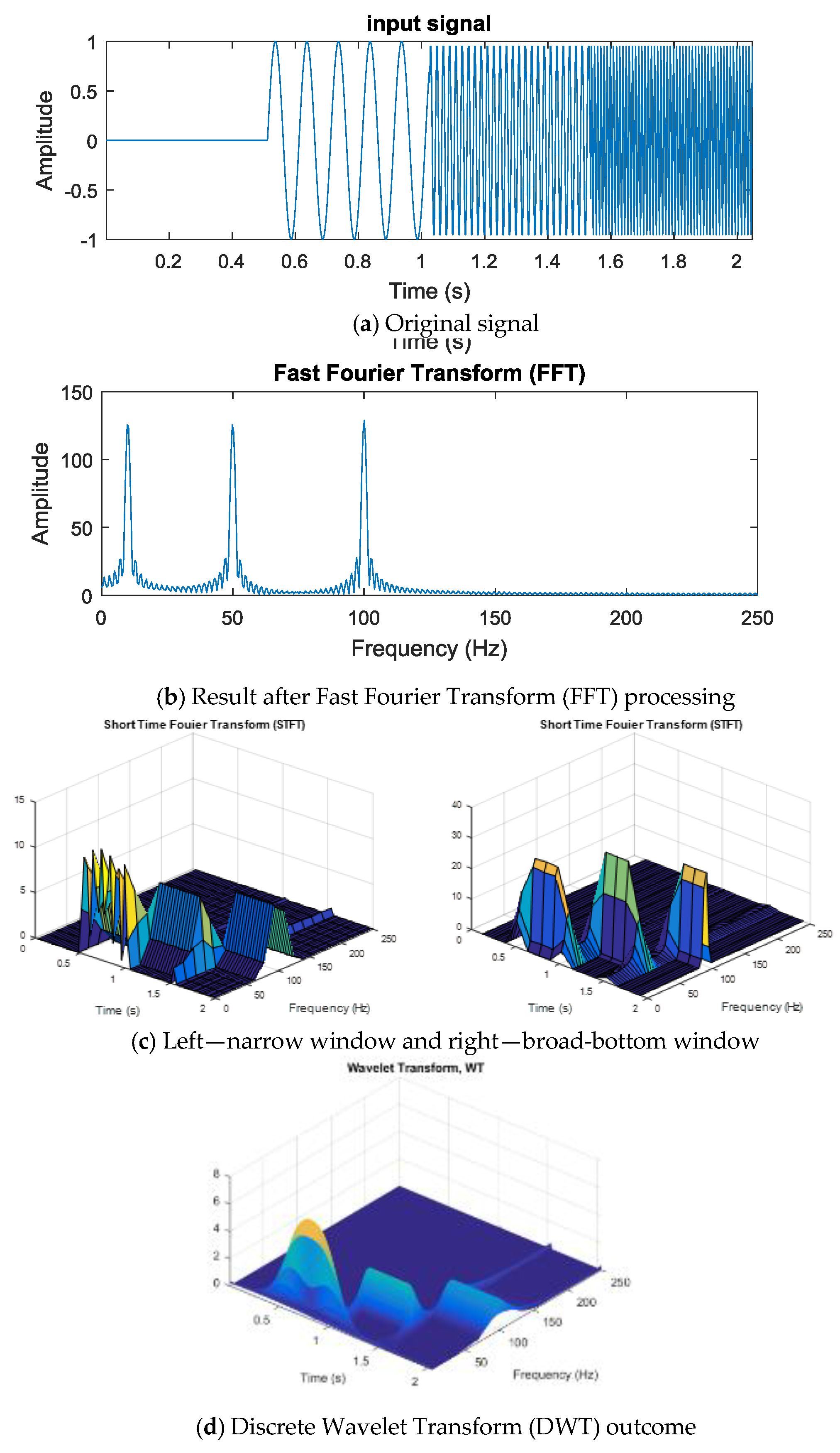
FFT, STFT, and DWT were introduced in the preceding paragraphs, and the three respective outcomes are now presented in
Figure 5. The input chirp signal is shown in
Figure 5a. It is obvious from
Figure 5b that FFT cannot present the linearity of a chirp signal. Furthermore, an apparent dilemma can be seen in selecting an appropriate window of analysis on time and frequency for STFT in
Figure 5c.
Figure 5d shows the wavelet transform that can be finally acquired.
2.4. Training and Classification of SVM, GRNN, and Deep-Learning-Based SDP
Classification is divided into two distinct steps: The first is to transform motor signals through the wavelet to compute their features. The features are thrown into SVM and GRNN for teaching and classification. The second step is to pictorialize and process the signals being transformed by the wavelet, and then to introduce the pictures into CNN for teaching and classification.
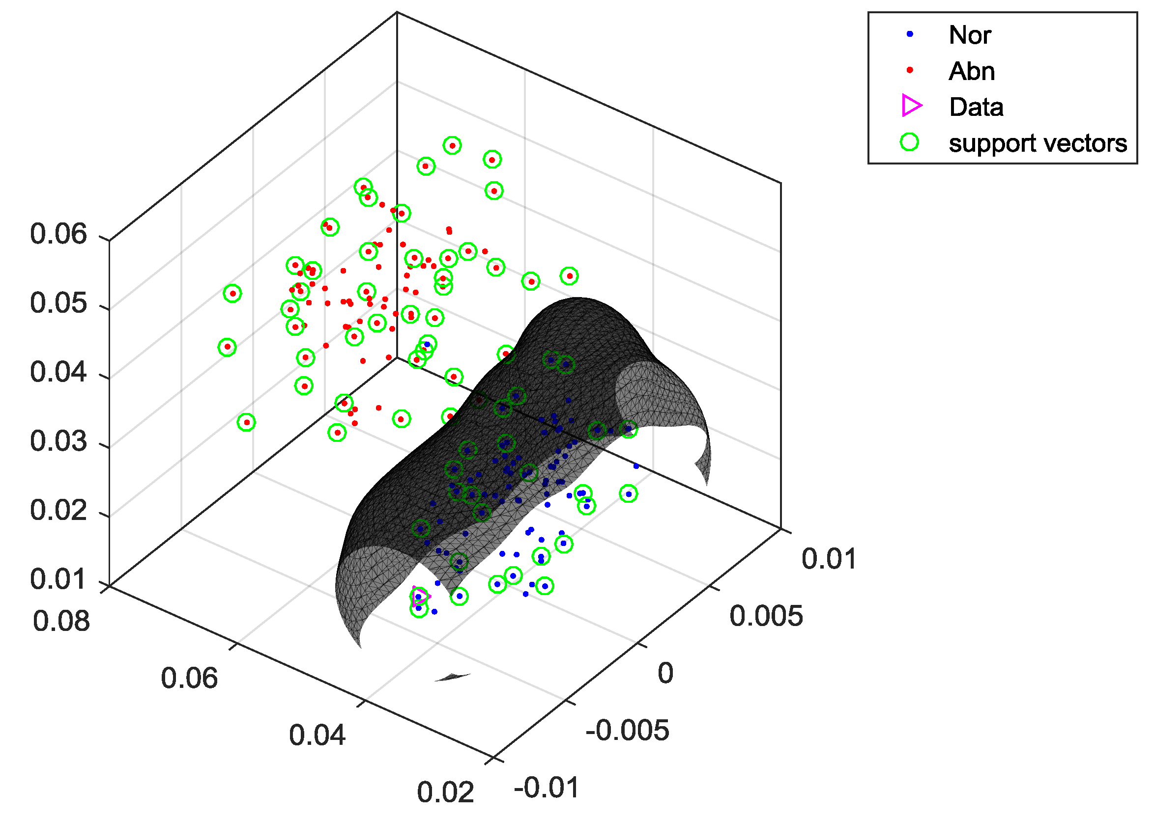
The main function of linear SVM is to find a hyperplane, which can separate the maximum margin from amongst all the input teaching data with diverse classification, where all the
located on the separating hyperplane satisfy the decision function, as shown in Equation (16):
where
w is the normal vector of this separating hyperplane, and
is the offset. When
, the datum is classified as
, and when
, the datum is classified as
. When the optimal separating hyperplane is found, the support vector must satisfy Equation (17):
where the distance of
is
, i.e.,
, and the margin is therefore
. When the maximum margin of the separating hyperplane is found, it is necessary to solve the minimum of
in compliance with Equation (17). The Lagrange Multipliers can be used to handle this optimization problem. The formula is as in Equation (18):
where
is the Lagrange coefficient, and
. According to the Karush–Kuhn–Tucker (KKT) Theorem, the optimum solution
can be substituted into Equation (18), to get Equation (19):
Any
satisfying Equation (19) is the answer for the support vector that is closest to the separating hyperplane. From all the above, it is possible to obtain the classification process function:
However, not all the data are helpful for finding the linear separating hyperplane in actual practice. It is necessary to map the original data to a higher-dimensional feature space through a nonlinear mapping function, , and then to implement linear classification from this feature space. If the mapping of the data is launched into a feature space, then the data will be . However, a kernel function can be used to replace , so it may not be necessary to first map the data to a feature space if the inner product of the data in the feature space can be resolved through the kernel function. The usual kernel functions include a linear, polynomial radial basis function (RBF), as well as a Sigmoid function. RBF was used in this study because the radial function is capable of sorting nonlinear data of high-dimensionality, and only two parameters need adjustment.
The very principle of GRNN is the regression of a dependent variable
on an independent variable
, which is then described through a probability density function (PDF). This differs from traditional regression analysis, which requires the initial assumption of a definite function. If
is the PDF for both variable
and
, and
x is an observed value of
, then the regression of
at this
x is as shown in Equation (21) [
17]:
Since
is still unknown, the observed values of both
and
are needed to estimate
. The Parzen window is used to measure
, and the result is shown in Equation (22):
where
is the dimension of
,
and
are the sample observed values
, n is the sample size, and
is the smoothing parameter, which is the only parameter to be configured in GRNN, and is usually between 0 and 1. We can therefore attain Equation (23) by substituting (22) into (21):
After simplifying Equation (23),
can be set, and the estimated observed value
y is as shown in Equation (24):
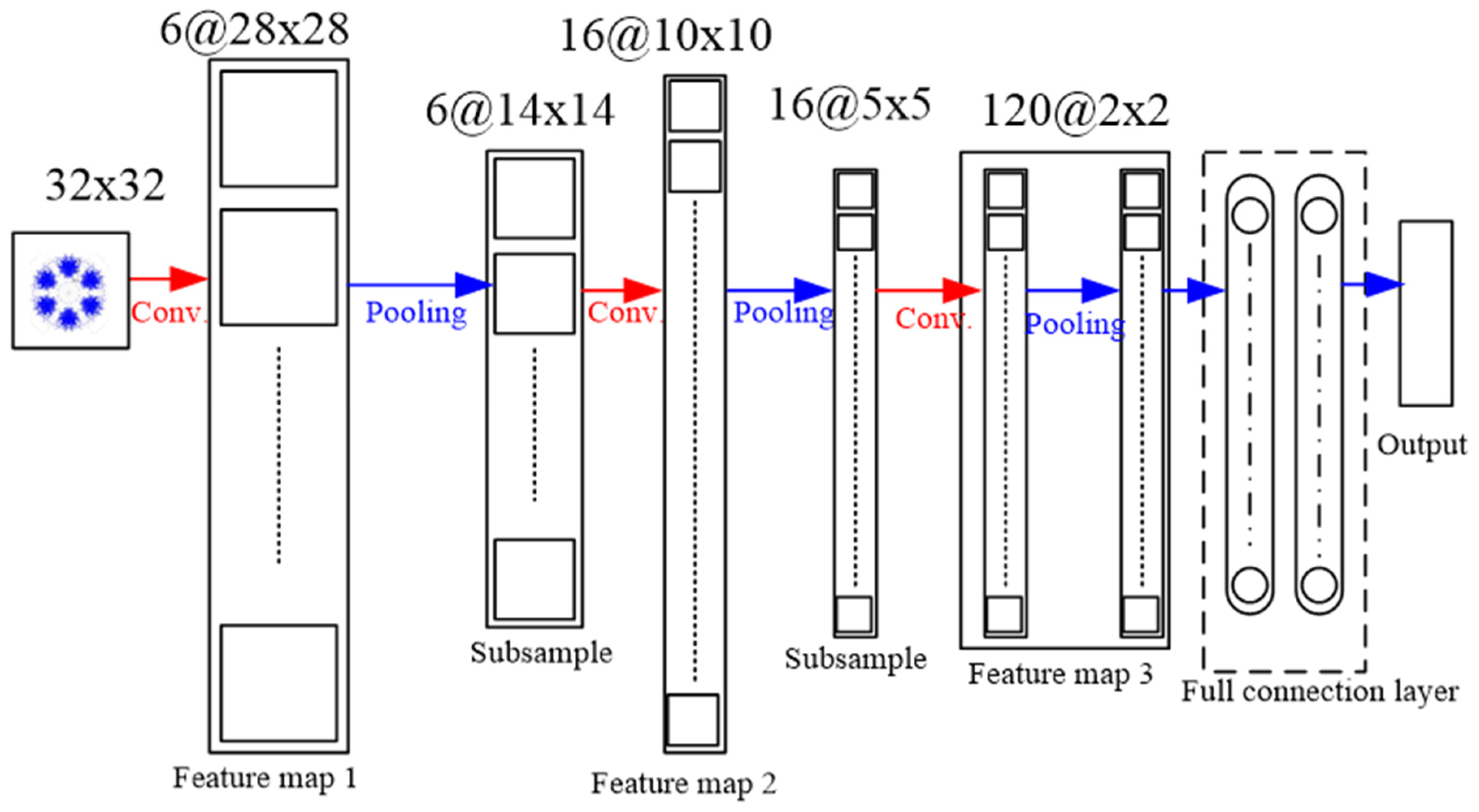
A Convolution Layer uses the local feature of a picture acquired by sliding from the left to the upper right, and then to the bottom through a window of fixed size. This becomes a feature as the next pooling layer; the sliding window is the convolution kernel. After the convolution kernel feature is obtained, the pooling layer is entered. The purpose of this is to lower the dimension of each feature map and retain its most important features. The pooling layer downsizes the scale of an input picture and also draws out the feature. The most usual pooling kernel scale is
, and the step length is 2. There are three major pooling-layer methods: max-pooling, mean-pooling, and stochastic-pooling. The final one is a fully connected layer, a general neural network, which flattens the feature information and connects to the neural network for classification [
18,
19].
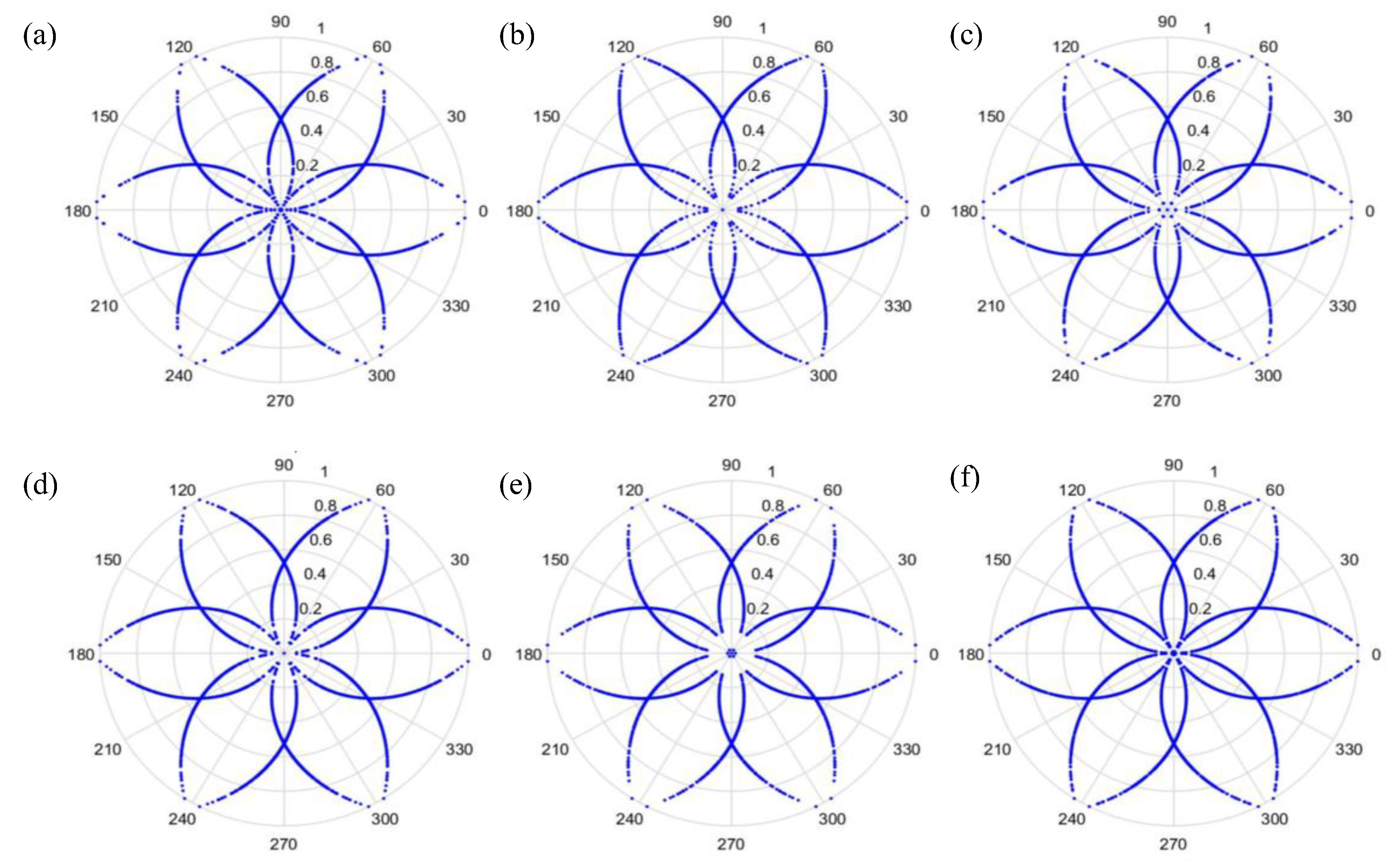
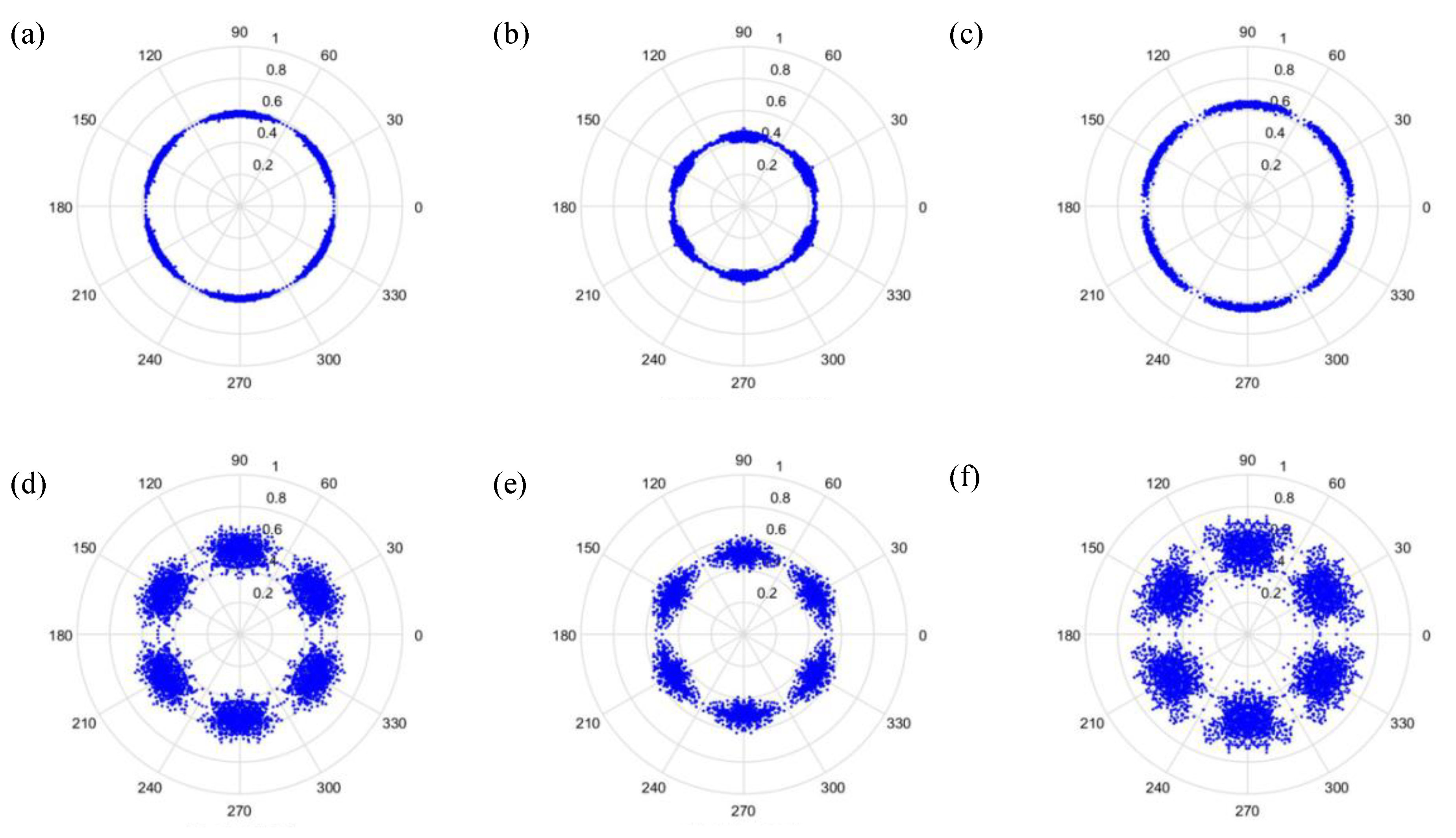
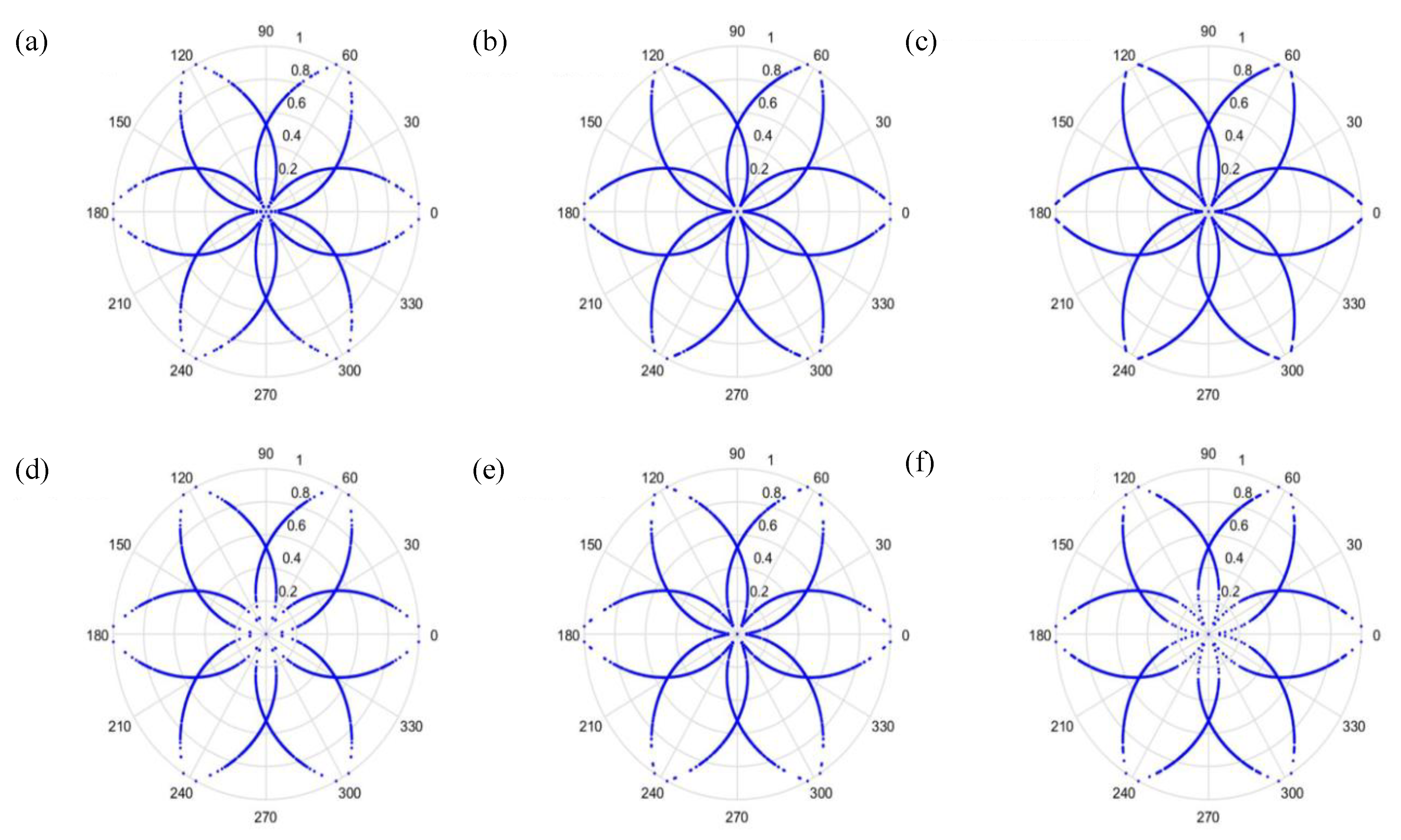
In this study, the signals were pictorialized, after which CNN was used to classify them. To do this, a map of symmetrized dots was used, as was done by Pickover [
23] for the visual characterization of speech waveforms. Pickover thought that it would be rather difficult to read all the data in numeric or character form. However, if the data were represented as a graphic, with a recognizable pattern, it could be more easily appreciated and understood. The basic principle of symmetrized dot pattern (SDP) technology is the mapping of the time waveform to polar coordinates to generate a map of dots. The dots are the time waveform and are mapped to the radial component, and the angular component is mapped by adjacent dots. The transform formulas are shown from Equations (25)–(27):
where
is the input signal,
H and
L are the maximum and the minimum of F, respectively,
is the rotational angle of the initial line,
is the signal gain, and
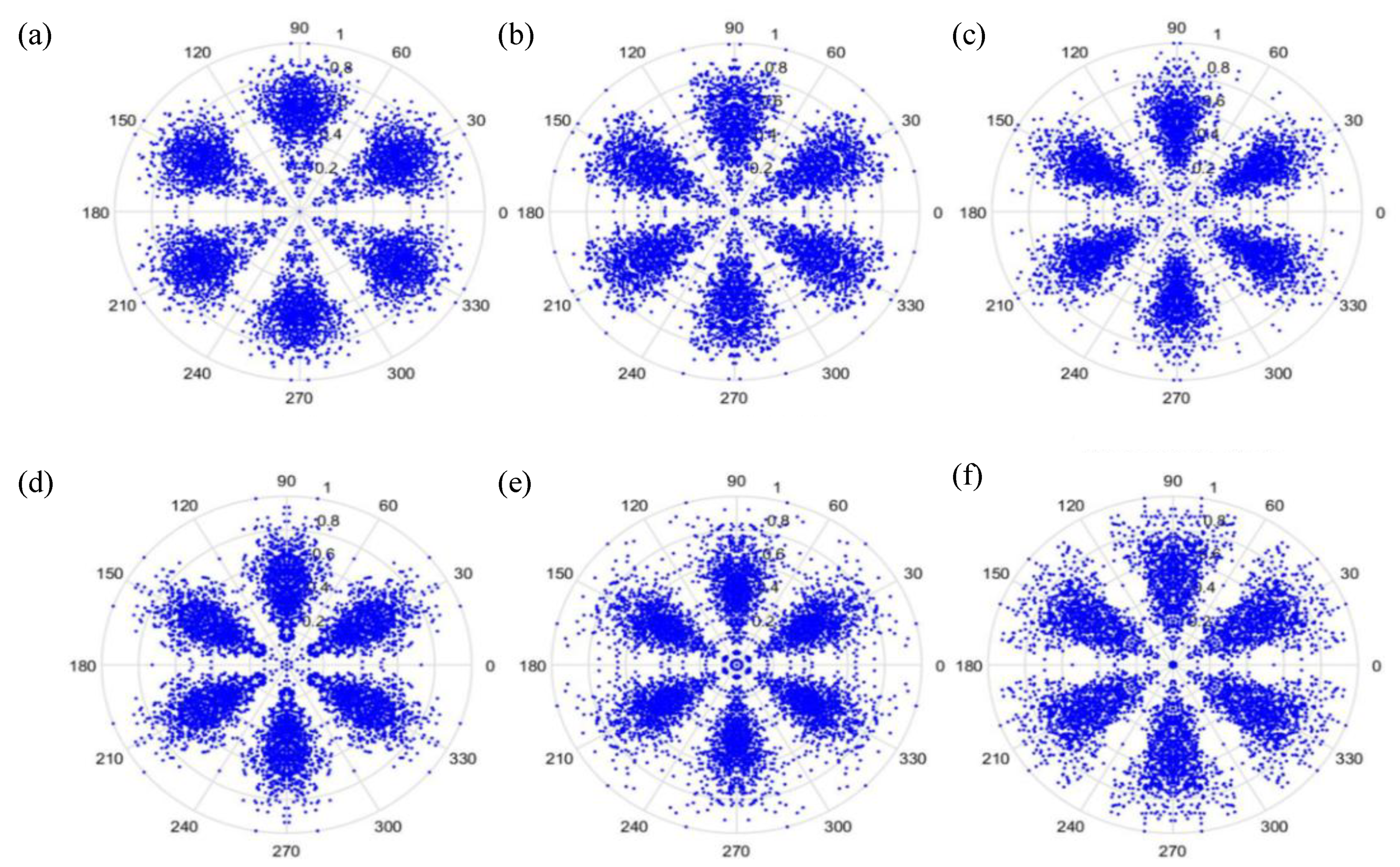
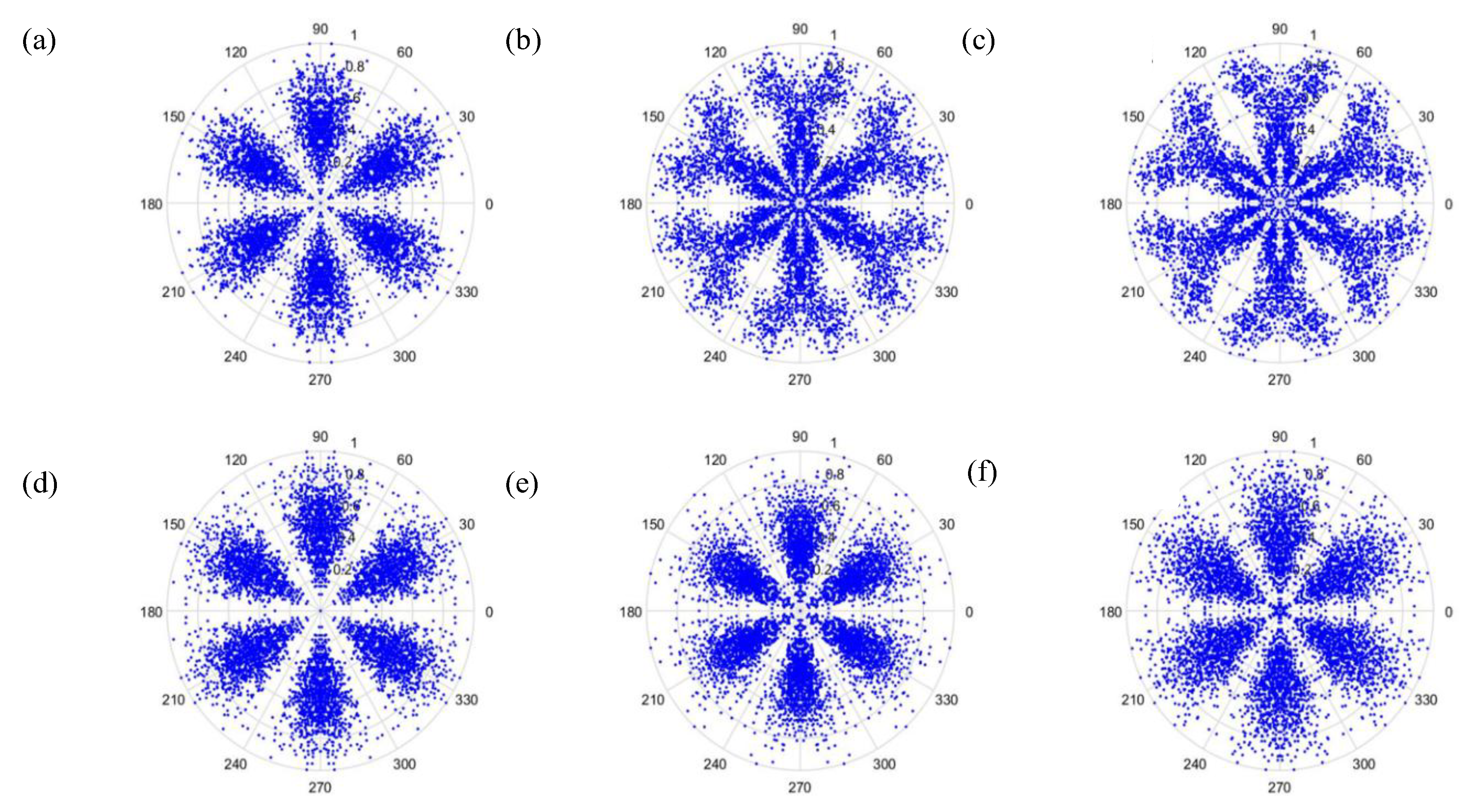
t is the time-lag coefficient. When parameter
t is changed, the outcome is shown in
Figure 6 and
Figure 7, when
t is 0 or 1, respectively.
As can be seen from
Figure 6 and
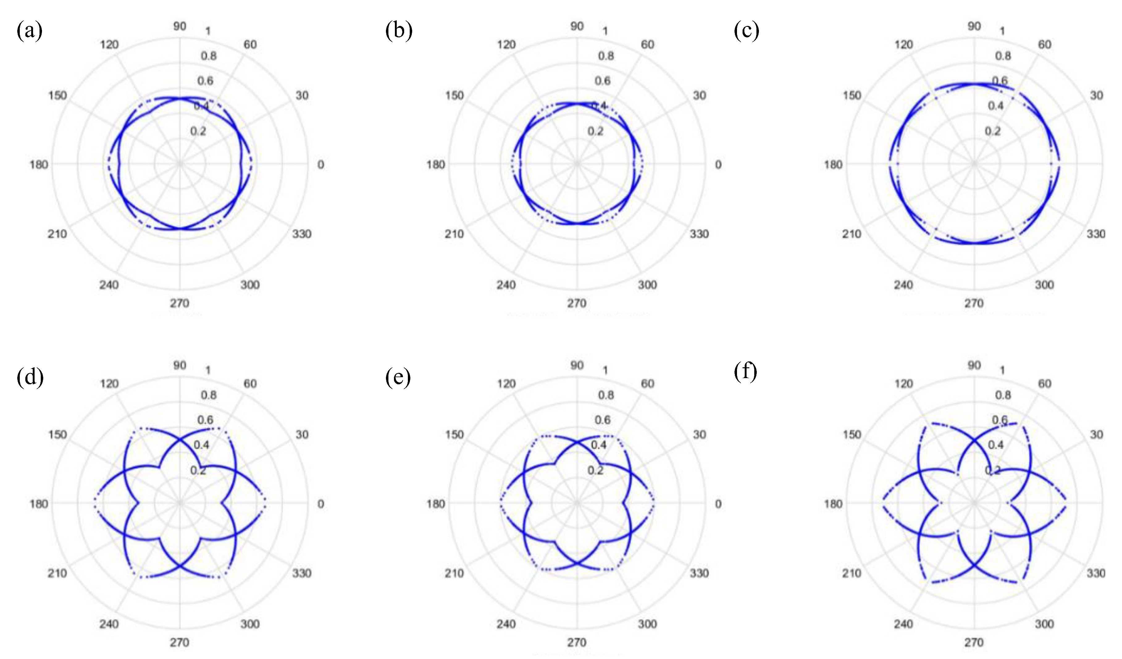
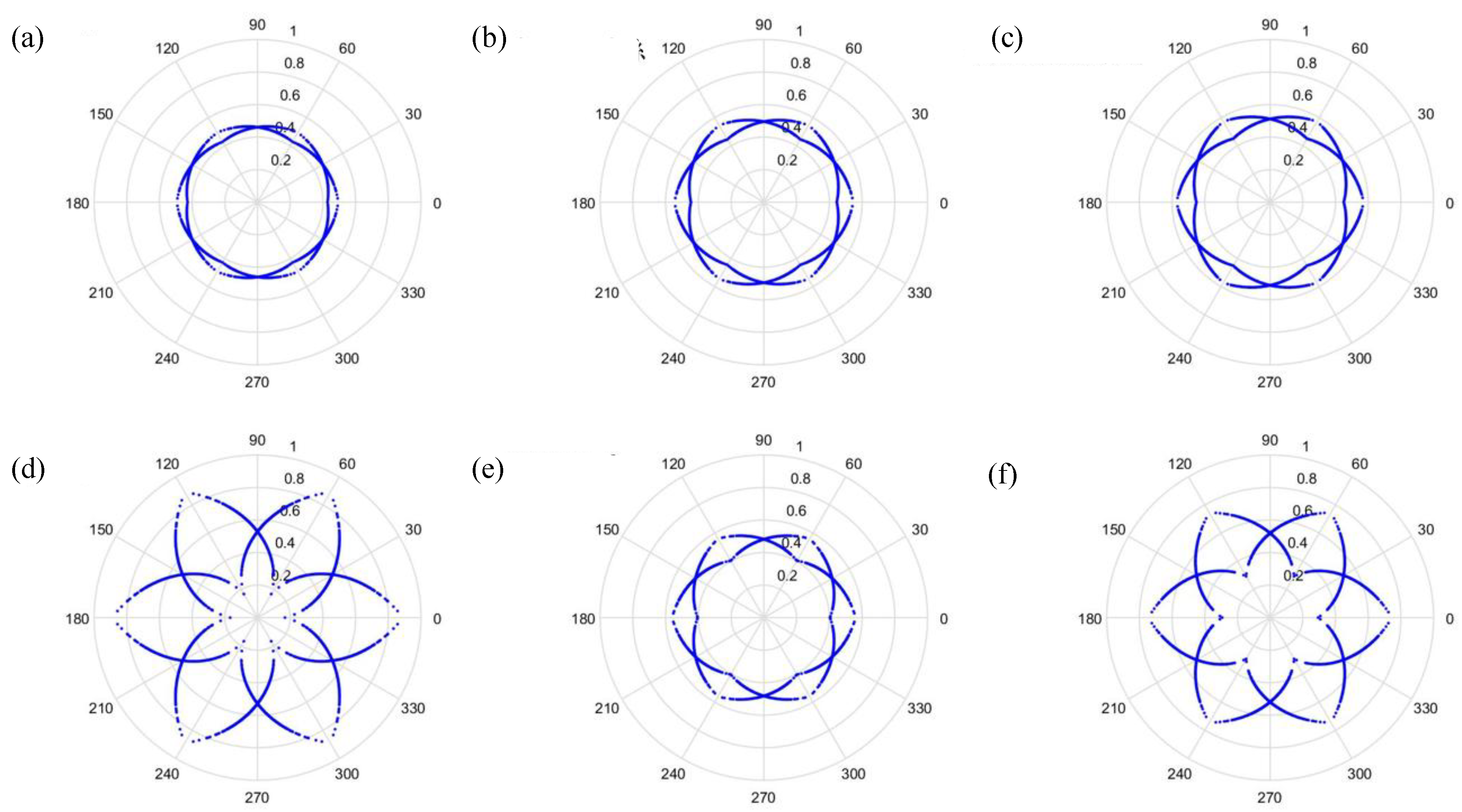
Figure 7, the dots are over-dispersed, and it may be difficult to spot the features of this picture via deep learning (DL). Furthermore, the maximum value,
H, in the experimental data is between 0 and 1, and the minimum value,
L, in the experimental data is between 0 and −1, and the answers gained from the formula
are located between 0 and −1. In addition,
are mostly known values to the second decimal place, and, as a result, the value of
is almost determined by
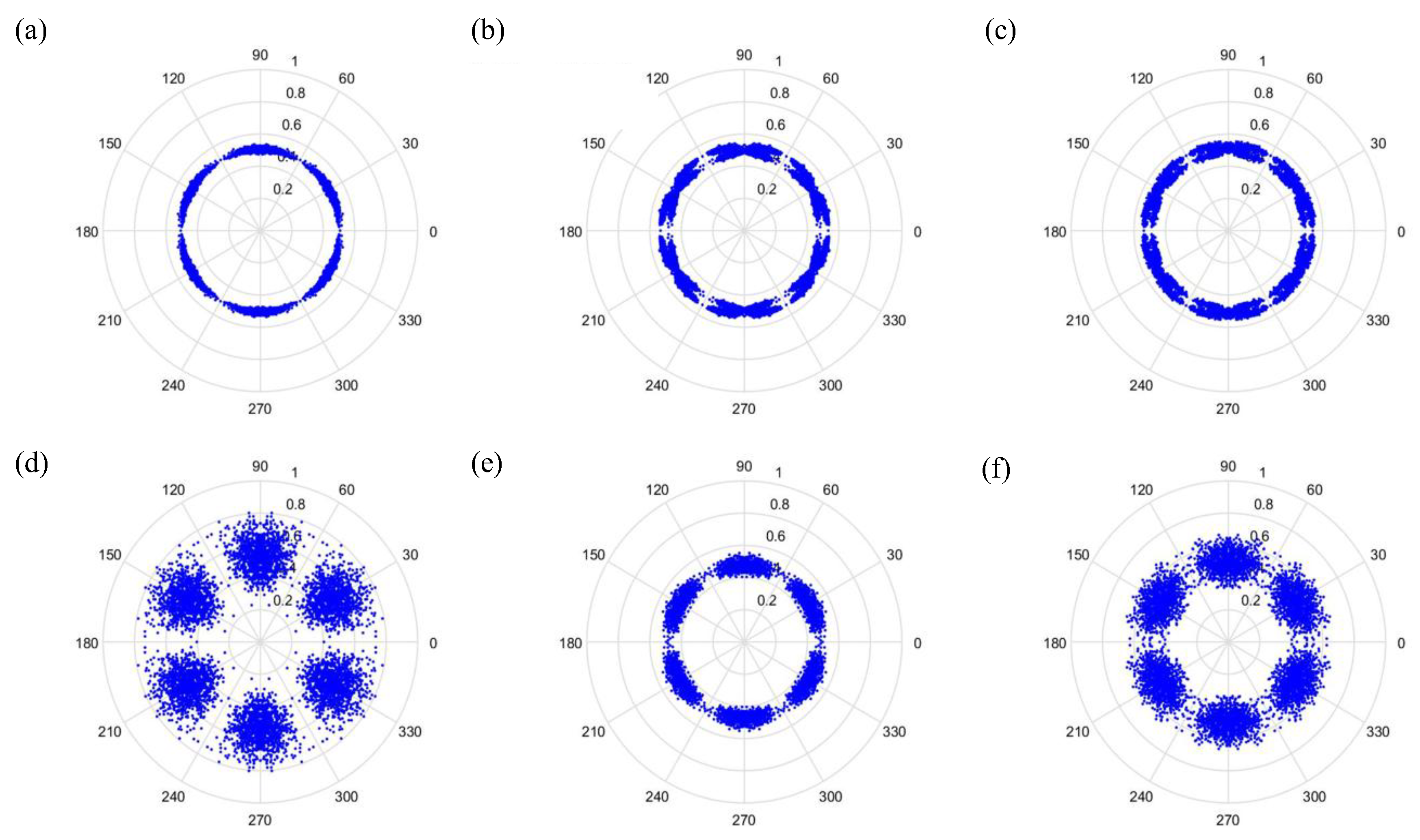
. The signal features can be fixed within a certain scope, in order to allow the dots in the picture to concentrate and be representative of the features, to allow better CNN identification. The radius after adjustment is shown in Equation (28), and the results are shown in
Figure 8 and
Figure 9.


