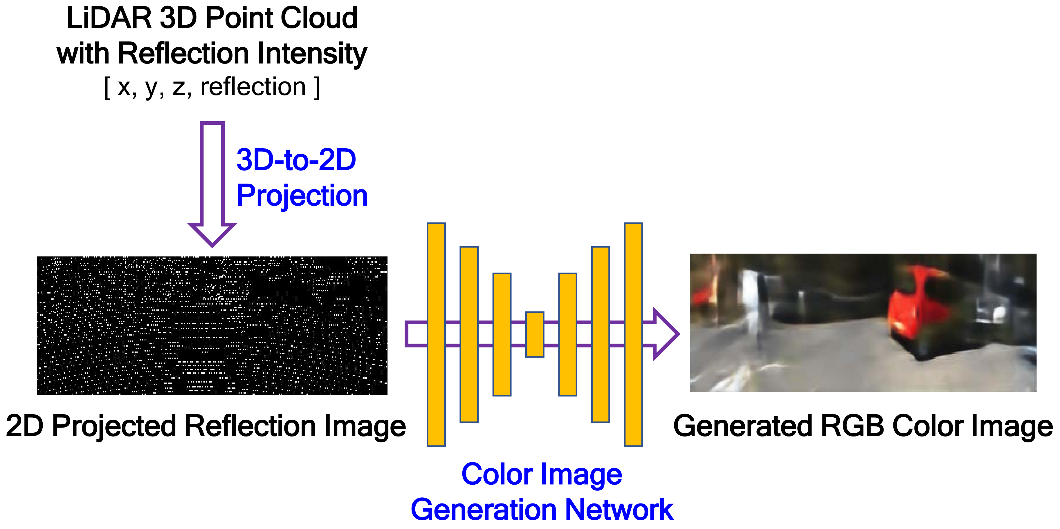
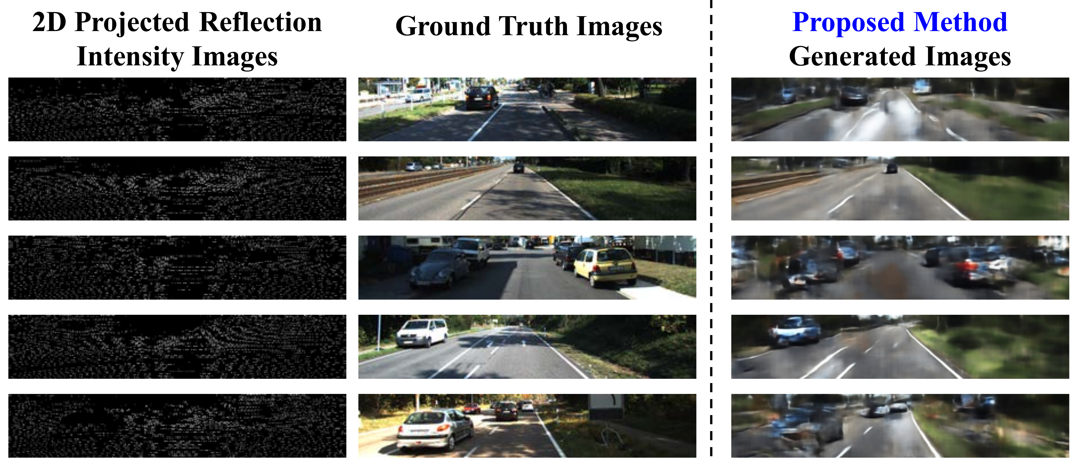
The proposed color image-generation system from LiDAR reflection intensity is composed of two steps: 3D-to-2D projection and color image generation, as shown in
Figure 2. The 3D-to-2D projection reconstructs a 2D projected reflection image by projecting the LiDAR 3D reflection intensity onto the target image plane desired. The projected reflection image is very sparse, as shown in lower left picture of
Figure 2, because of the different resolution and field of view (FOV) between LiDAR and the target image. The target image is assumed to have the same image plane that is captured by a camera installed on the vehicle. The goal of our work is to generate a color image that is as similar as possible to the image captured by the camera from the LiDAR 3D reflection intensity. In the image-generation step, RGB components are generated from the 2D reflection image using the encoder-decoder-structured FCN model. Unlike the conventional FCN application, the color image should be generated from the sparse 2D reflection image. This is why the proposed FCN is designed to have an asymmetric network structure, i.e., the layer depth of the decoder in the FCN is deeper than that of the encoder.
In the following subsection, we describe in detail the 3D-to-2D projection and color image- generation network. In addition, the training and inference processes are also described.
3.2. Proposed Color Image-Generation Network
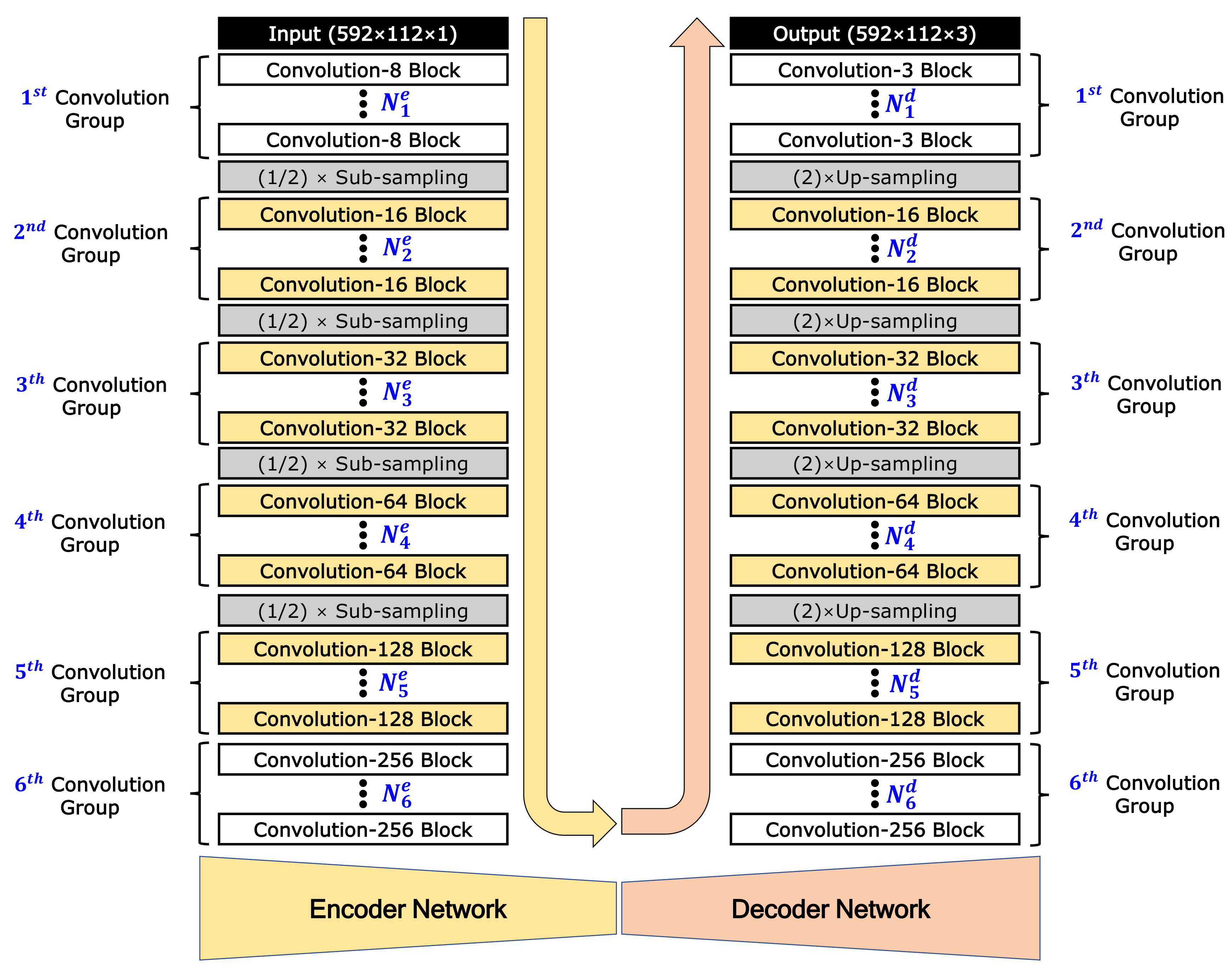
The proposed color image-generation network model is designed with an asymmetric encoder-decoder-structured FCN model as shown in
Figure 3. This model generates a color image with 3 channels (size: 592 × 112 × 3) from the sparse 2D reflection image with 1 channel (592 × 112 × 1). The encoder network consists mainly of several convolution blocks and sub-sampling steps. Each convolution block is composed of a convolution layer, batch-normalization layer, and activation function, in consecutive order. The decoder also consists of several up-sampling steps and convolution blocks. As various numbers of convolution blocks can be applied before each sub-sampling or up-sampling, we introduce a new terminology called the convolution group, which consists of several convolution blocks. In this work, considering the size of the input and output images, the encoder network is designed with six convolution groups and four sub-sampling steps. The decoder is designed with four up-sampling steps and six convolution groups. In
Figure 3,
and
represent the number of convolution blocks in the convolution group of the encoder and decoder, respectively. As results, the number of convolution blocks is
and
in the encoder and decoder networks, respectively. For sub-sampling, max-pooling with a factor of 2 is applied. For up-sampling, un-pooling [
35] with a factor of 2 is applied. In each block,
K convolution layers are applied, which is denoted as the convolution-
K block. According to the research results that indicate that dropout is not needed when using batch normalization [
32], dropout is not applied in the proposed network.
Whereas the convolution-8 block is applied in the first convolution group of the encoder, the convolution-3 block is applied in the last convolution group of the decoder because the output is a 3-channel color image. In all the convolution layers, stride 1 and the same zero padding are applied. Except for the convolution-3 blocks of the last convolution group in the decoder, a rectified linear unit (
) is used for the activation function in all convolution blocks. In the last convolution-3 blocks, hyperbolic tangent (
) is used for the activation function and batch normalization is not applied. The
and
functions are as follows:
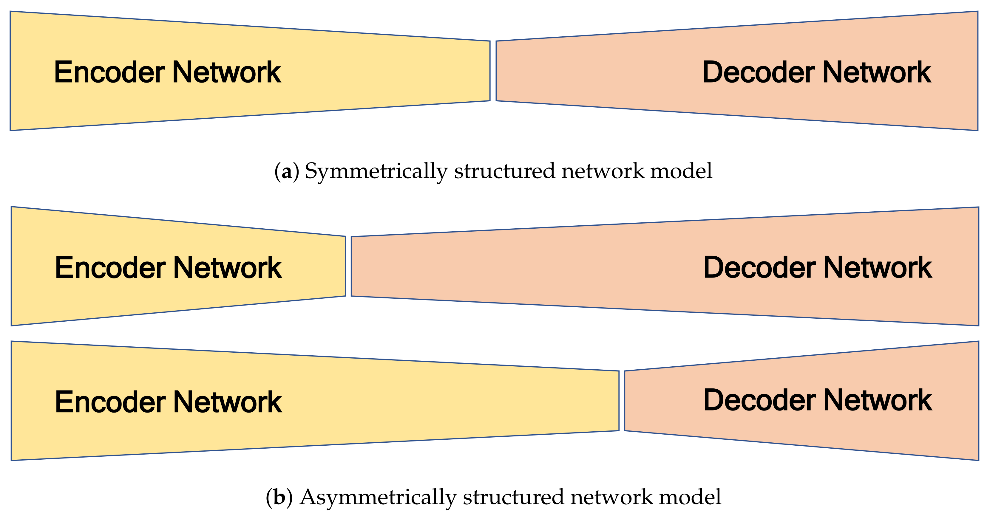
The role of the encoder network is to extract features from the sparse 2D reflection-intensity image. The role of the decoder network is to map the low-resolution feature maps to an RGB color image with full output resolution. Because the projected 2D reflection and generated color images have different amounts of information, it is necessary to apply different numbers of convolution blocks in the encoder and decoder. The proposed network can be regarded as a symmetrically structured FCN when it has the same the number of blocks between the
ith convolution groups in the encoder and decoder (
) as shown in
Figure 4a. An asymmetrically structured FCN can be realized if the
ith convolution groups in the encoder and decoder have different numbers of block (
).
Figure 4b shows two cases of asymmetrically structured networks: the first is the case of a decoder that has greater depth than the encoder (
), and the second is the reverse (
).
The total number of layers in the proposed network is obtained by summing the number of convolutions and batch-normalization layers in both the encoder and decoder. As each convolution block consists of one convolution and one batch-normalization layer, the number of layers at encoder
and decoder
are calculated as follows:
Note that batch normalization is not performed in the last convolution block of the decoder. Therefore, the number of total layers
is calculated as follows:
Assume that all convolution filters used in the proposed network have the same size (
). As all convolution blocks in the
ith convolution group have the same number of convolution filters, each block belonging to the
ith group has
(or
) convolution filters in the
ith group of the encoder (or decoder). The total number of parameters is obtained by summing the number of weights and biases of the convolution layers and the number of parameters of the batch-normalization layers. The number of parameters at encoder
is calculated as follows:
At the decoder, the number of parameters
is given by:
In Equations (
6) and (
7), the first and second terms on the right side indicate the number of weights and biases in the convolution layers and the third term is the number of parameters in the batch-normalization layers. Therefore, the total number of parameters in the proposed network
is given by:
As mentioned before, the number of convolution filters in the first group of the encoder and the last group of the decoder are fixed to eight and three, i.e., and . For other groups, we design that the number of convolution filters is increased by a power of two (, for ). All convolution filters are designed to be of (3 × 3) size ().
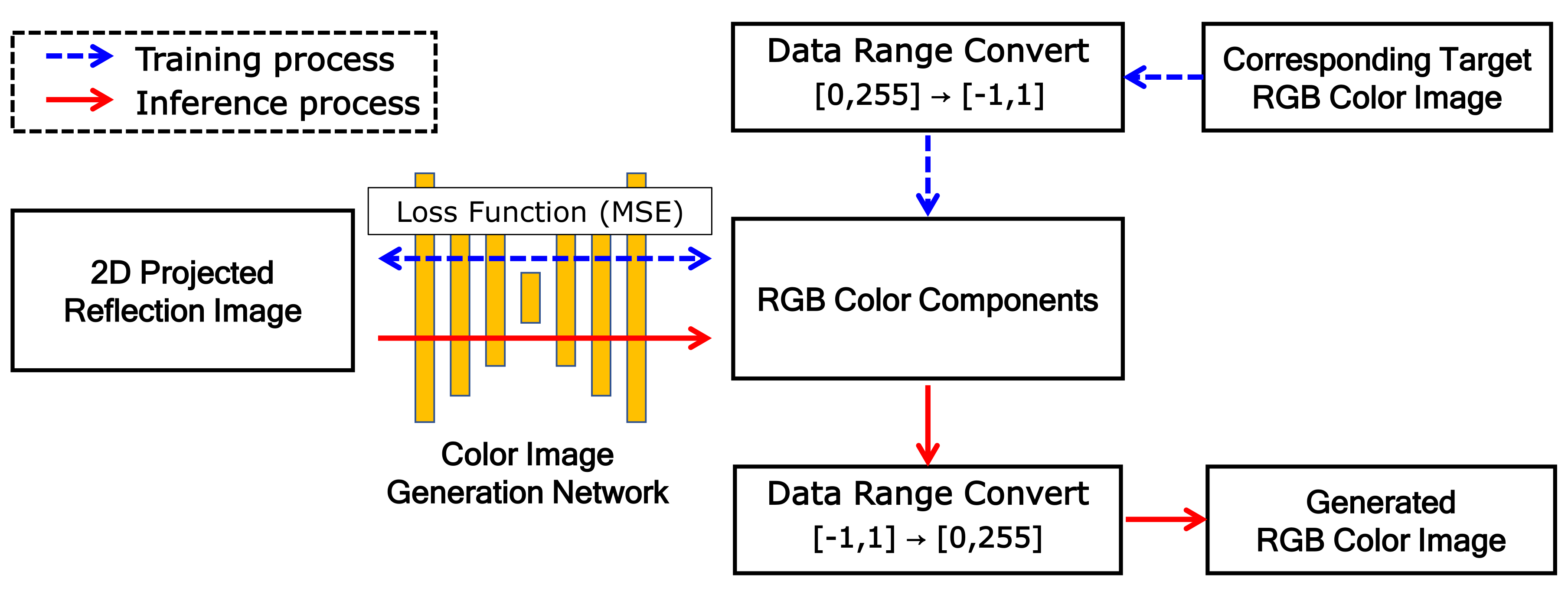
3.3. Training and Inference Processes
Figure 5 shows the training and inference processes of the proposed network. The training process is indicated by blue dashed arrows and the inference process by red solid arrows.
In the training process, the 2D projected reflection-intensity image and corresponding RGB color image are used as the dataset. The projected reflection image is used as input for the proposed model and the corresponding color image is used as the target image that is the ground truth (GT). Because the
function is used as the activation function of the last convolution group, the dynamic range of the output image to be generated is
. Thus, the GT color image is converted to the same dynamic range, where each color component is mapped to the dynamic range independently. The loss function is mean-squared error (MSE) between target
T and generation
G images, as follows:
where,
m and
n are the width and height of the image and
c indicates the number of channels.
In the inference process, RGB components are generated through the proposed color image-generation network with training parameters. As the RGB components have a dynamic range of , the final generated RGB color image is obtained by conversion to the range of .


