2.1. Overview
To improve GNSS measurement and positioning accuracy in GNSS challenged environments, a deeply-coupled receiver with adaptive open-close tracking strategy and INS aided pseudo-range weight control algorithm is proposed based on the non-coherent deep couple structure in [
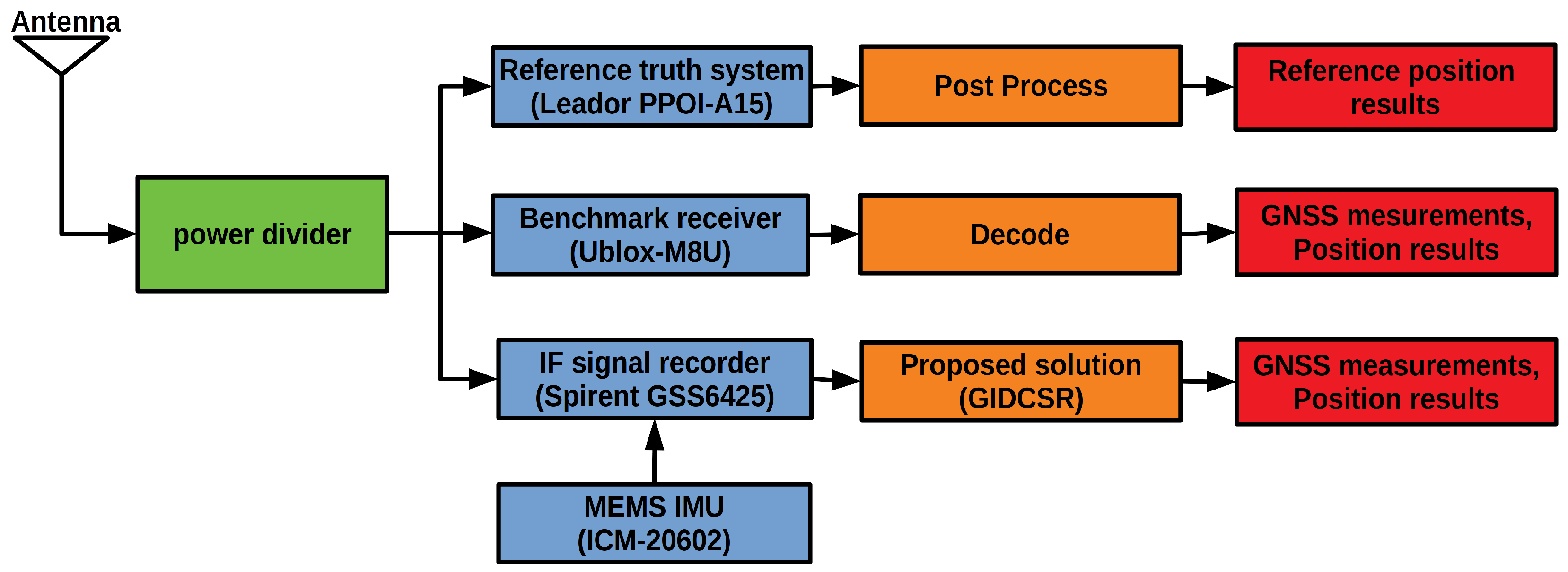
43]. The GIDCSR architecture is shown in
Figure 1. The architecture is composed of three blocks which are the GNSS signal processing module, the INS module and the integration filter. GNSS signal processing module is in charge of the processing of GNSS intermediate frequency (IF) signals, producing GNSS observations. INS block mainly presents the position and velocity information of the vehicle in a high frequency. A GNSS/INS integration algorithm based on Kalman filter is performed in the integration filter to provide the final navigation results and IMU errors. The INS predicts the move Doppler of the vehicle and feeds it to the NCO control algorithm. The adaptive tracking is capable of extracting carrier phase when GNSS signals are in good condition. It can also avoid the impact of loop filter output deterioration on NCO control to ensure the quality of pseudo-range and Doppler. Other than that, the proposed MEMS INS aided weight control algorithm will suppress the deterioration of pseudo-range accuracy caused by signal attenuation and multipath, thereby helping to improve the quality of NCO control information and deep couple positioning accuracy in GNSS-challenged environment.
An antenna receives the GNSS signals and feeds them to a radio frequency(RF) front end in which the GNSS signals are down converted to IF signals, which can be expressed as follows [
45,
46]:
where
A is the amplitude of IF signal,
and
are the Pseudo Random Number (PRN) code and navigation data bit respectively.
is the IF frequency,
is the Doppler frequency, and
is the initial phase. We use
as the noise of IF signal which is modeled as zero-mean white Gaussian noise (WGN). The subscripts
I and
Q represent the in-phase and quadrant-phase signals respectively.
The IF signals go through a mixer and a correlator, producing the correlated signals. Then an integration and dump operation is performed, the results have the following form:
where
is the coherent integration time,
is the Doppler estimation error, and
is the initial phase estimation error. Note that the period of the integration can be no longer than a navigation bit because of the bit hopping. The measurement pre-processing operates on the accumulated correlator outputs and then it performs the discriminator function to form Kalman filter measurements.
A MEMS IMU is employed to estimate vehicle movements in the GIDCSR. Its bias and scale-factor errors are included in the functional model of the IMU and are estimated by the GNSS/INS integration filter. The error model of the IMU is expressed as:
where
and
are raw output of the IMU. We use
and
to denote the truth value of the angular velocity and specific force.
and
are the biases of the gyroscope and accelerometer respectively.
and
are scale-factor errors.
is the noise. In the GNSS/INS integration filter, the state vector has the following form:
where
,
,
are the position, velocity and attitude error, respectively.
In deeply coupled mode, the INS output is also used for motion Doppler prediction between vehicle and satellites to assist GNSS tracking loops [
18]. With the predicted motion Doppler, along side with the receiver clock noise estimation presented by the integration filter, the tracking loops need only to tolerate the INS estimation error, instead of the vehicle dynamic. In other words, the tracking loops can work under a quasi-static situation, which permits us to compress the bandwidth and lengthen the integration time to suppress thermal noise.
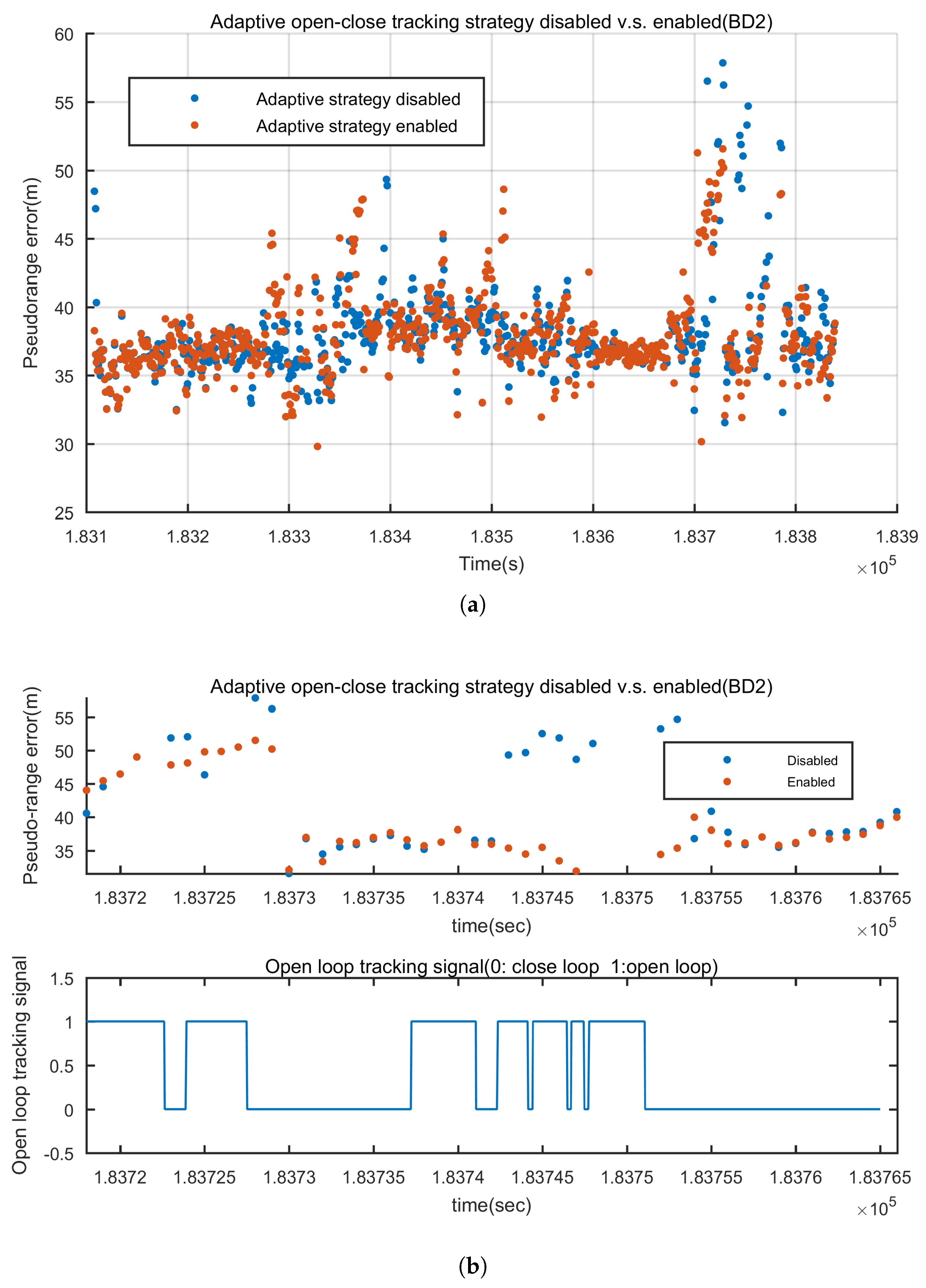
In order to improve the performance of the tracking loops in GNSS-challenged urban environments, with the INS assistance, an adaptive open-close loop strategy is applied, which plays a significant role in the GIDCSR. This strategy permits each channel to switch between open-loop and closed-loop tracking adaptively, improving the accuracy and robustness of tracking loop greatly. After a Fast Fourier Transform (FFT) operation on the integrated signals, an FFT-based signal-to-noise ratio (SNR) indicator is calculated. Compared with carrier-to-noise ratio (CNR), the FFT-based SNR is calculated in a higher frequency and is more robust. According to the FFT-based SNR, the receiver determines whether to cut-off the loop filter to NCO switch. If the signals are too weak or the loop loses lock, the switch is cut off and an open-loop tracking of the signal is applied. If all the satellite channels are in closed-loop mode, the GIDCSR is a classic GNSS/INS scalar-based deeply coupled structure [
47]. When all the channels are in open-loop mode, the GIDCSR works as a GNSS/INS federated vector-based deeply coupled structure [
43]. Therefore, with the proposed adaptive open-close loop strategy, the GIDCSR can change between scalar and vector structure flexibly. When the GNSS signal is strong, the channel in closed-loop mode can track the carrier phase accurately. When the GNSS signal is attenuated, blocked or reflected, the channel in open-loop mode can track the pseudo-range robustly.
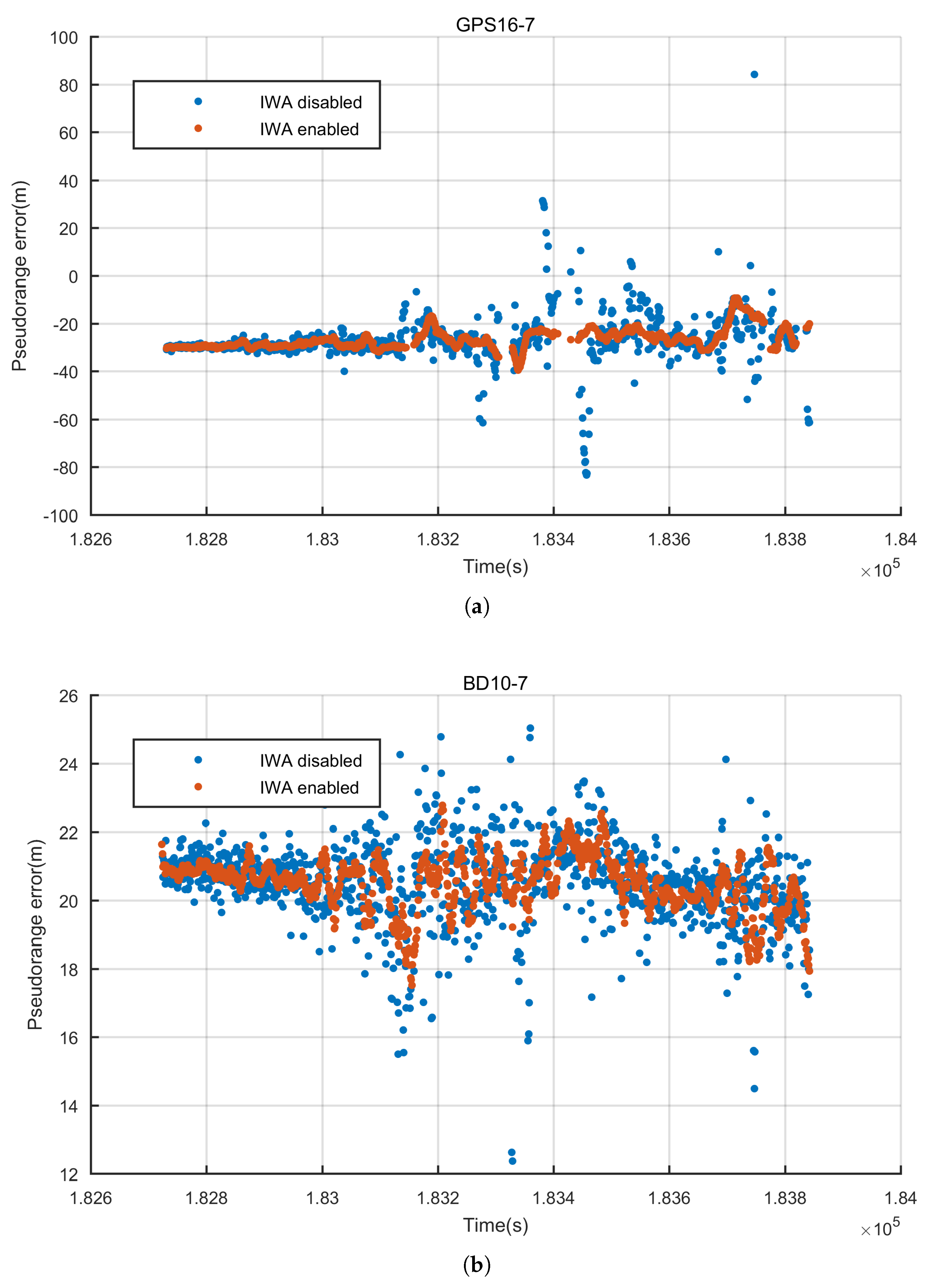
In addition, we propose an INS Aided Pseudo-range Weight Control Algorithm (IWA) to eliminate the pseudo-range gross errors caused by attenuated, blocked or reflected GNSS signals. The GNSS/INS integrated navigation position of last epoch is used to estimate the distance between the vehicle and each satellite. Then a reference satellite is chosen and a double-difference alike operation is performed. By this way, the errors of the pseudo-ranges can be estimated and applied to weight the pseudo-ranges. A detailed description will be provided later. It turns out that IWA can improve the quality of the pseudo-ranges and position greatly in GNSS-challenged environments.
2.2. Adaptive Open-Close Loop Strategy
In urban environments, GNSS signals are frequently reflected, blocked and weakened. When the signals are too weak (basically with CNR lower than 20 dB-Hz) or blocked, the discriminator outputs cannot truly reflect the difference between NCOs and input signals, caused to incorrectly control NCOs. A common strategy in a pure GNSS receiver is to announce the tracking loop loses lock and a reacquisition is performed. This way of tracking recovery is neither fast nor accurate, and it will be nearly useless when the signals are blocked frequently, which is very common in urban environments.
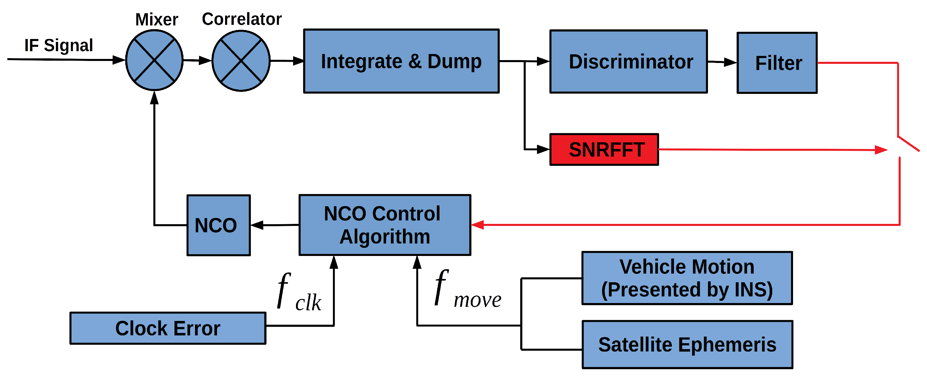
This paper presents an open-close loop strategy to overcome the problem, shown in
Figure 2. With the vehicle position presented by INS and the satellite position, the line-of-sight unit vector of the vehicle relative to the satellite is calculated in the first place. Then the line-of-sight motion Doppler
is calculated according to the vehicle velocity and satellite velocity. Every time the Kalman filter is updated, the frequency deviation of the receiver clock
is estimated. When SNRFFT indicates strong signal strength, the Doppler error output by the local filter, the motion Doppler and receiver clock deviation jointly control the NCO in which the carrier phase can be extracted. When the SNRFFT results present unacceptable signal noise, the loop filter output is not sent to control the NCO, and only the motion Doppler and clock deviation are used to control the NCO, turning the tracking loop into an open-loop status. Three types of NCO control information can be updated in different frequency.
The strategy can improve the continuity of the signal tracking greatly. When part of the satellites are blocked, the INS errors can still be corrected by visible satellite, which means the aiding Doppler errors provided by INS will not diverge. Therefore, with the assistance of INS aiding information, the NCO error would not increase quickly. When the blocked satellites are available again, the tracking loop can recover accurate carrier phase tracking rapidly. In other words, the strong signal channels assist those channels with weak signals, which meets the philosophy of vector based tracking. This strategy combines the advantages of both scalar and vector based structures. When a channel is in closed loop, it can track carrier phase steadily. And when the signals are weak and frequently blocked, the open loop tracking can improve the robustness of tracking.
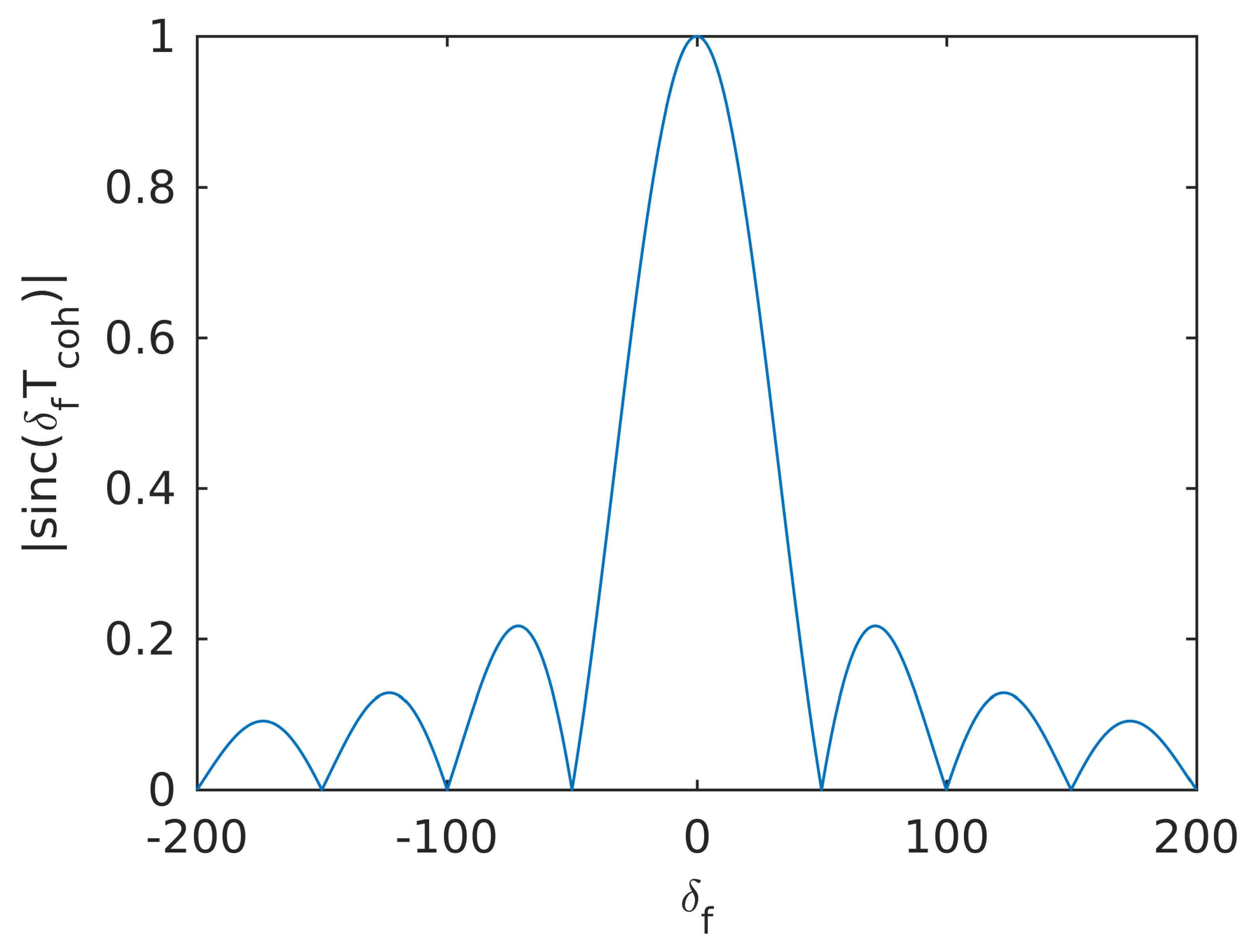
The traditional approach to estimate the power of GNSS signals is called the Narrowband-Wideband Power Ratio (NWPR) [
48]. NWPR calculates the ratio between wideband power (WBP) with bandwidth
and the narrowband power (NBP) with bandwidth
. Typically the
is set to 1 ms and
M is set to 20. This approach is sensitive to the Doppler estimation error because 20 ms integration time is used. When the coherent integration time is set to 20 ms, the relationship between the amplitude of the integrated signal and the Doppler error is shown in
Figure 3. The amplitude of the integrated signal drops to zero when the Doppler error is 50 Hz. We propose a faster and more robust FFT-based indicator is presented to outcome the shortcomings of NWPR.
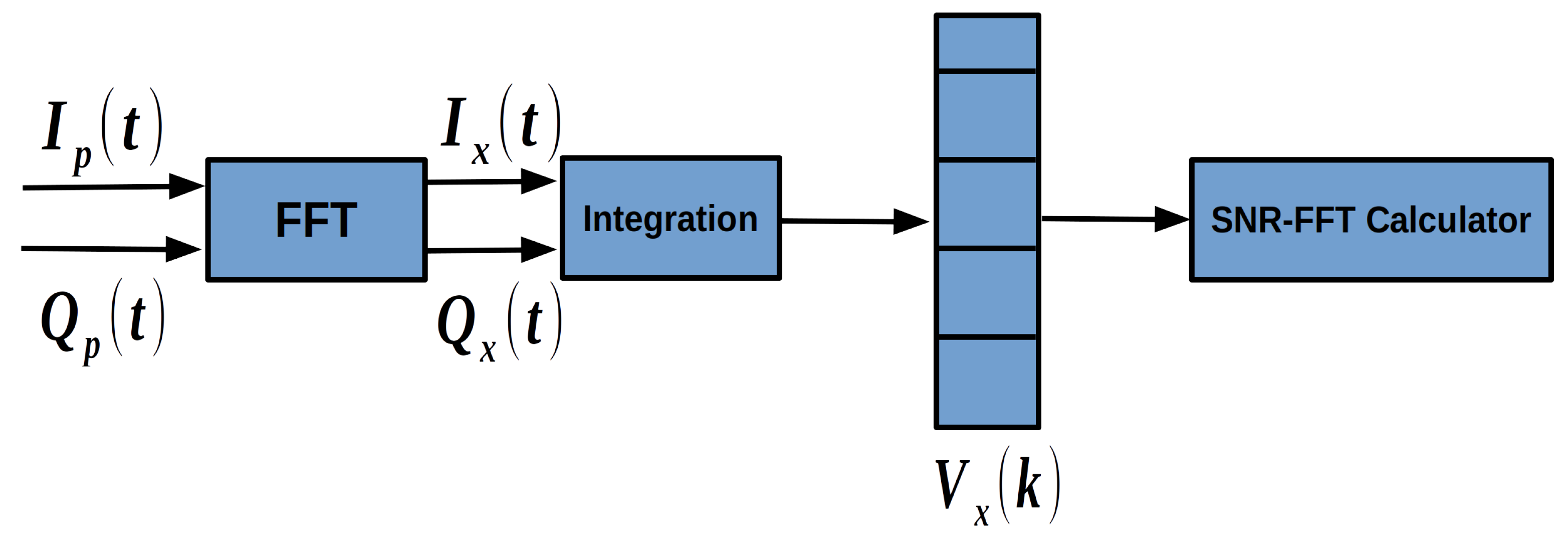
The scheme of SNR-FFT is shown in
Figure 4. SNR-FFT takes correlator integration results of GNSS signals
and
as input. The complex form of (
2) is as follows:
The discrete-time model of the accumulated signal over the
ith integration interval can be expressed as:
where
and
are the outputs of correlator and
epochs of data are accumulated.
The FFT operation can be expressed as:
where
is the time domain input signal,
is the frequency domain output signal and the subscript
x means the signal is converted to frequency domain. N is the number of FFT processing points.
The FFT result reflects the power density distribution with respect to the Doppler frequency residual. As is shown in (
5), the integrated signal is a single tone complex signal. Although the signal is flooded in the noise in time domain, the power of the single tone complex signal can stand out at the specific frequency point in frequency domain. Note that the FFT performs a series of multiplication and addition operations. Essentially the FFT method is equivalent to coherent integration. So the length of the input of the signals can be no longer than 20 ms because of the bit-flipping. The resolution of the FFT method
can be denoted as:
where
is the sampling rate and
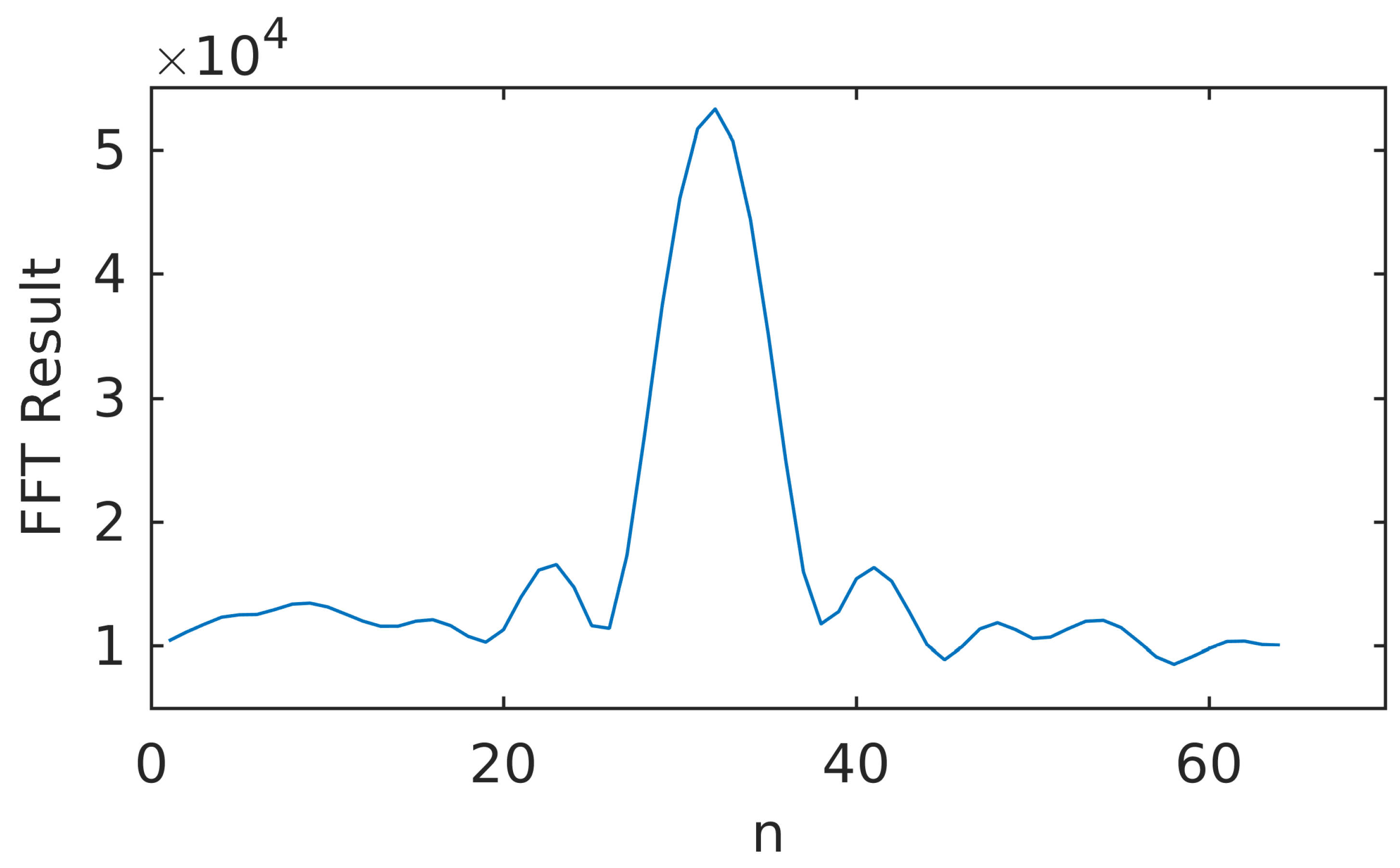
is the number of FFT processing points. Sometimes the signals can be weak and the peak of the FFT results is hard to detect, making it difficult to calculate the SNR-FFT indicator. To solve the problem, an accumulation function is performed on the FFT results:
where
FFT results are accumulated and
is the
mth FFT result in the accumulation interval with index
k. In this way the power of the signals are accumulated. The integrated FFT result is shown in
Figure 5. The peak is where the Doppler frequency residual stands. The rest is noise. We can see that the peak is not in a single frequency point. It is because that the resolution of the FFT method is not infinite. The power of the specific frequency point is spread to the several points near it. Let
denote the maximum energy,
and
denote the maximum energy adjacent to
. An FFT based SNR indicator can be calculated as:
where
is the total energy of signal and noise in the FFT bandwidth:
In (
10),
denotes the power of signal and
is the estimation of power of noise. The FFT based SNR can be calculated this way. SNR-FFT can detect very weak signals. Also it can reflect the change of satellite signal strength in a timely manner, so that the loop strategy can make corresponding adjustments in time. In GIDCSR, when the SNR-FFT detects a signal with
lower than 25 dB-Hz, which is set as the carrier phase tracking threshold, the open-loop tracking mode is turned on.
2.3. INS Aided Pseudo-Range Weight Control Algorithm
The common approaches to weight GNSS pseudo-range are based on signal
and satellite elevation, which are reasonable in open sky environments. In urban environments, these approaches are not suitable because of the existence of not line of sight (NLOS) signals and severe multipath [
49]. As a solution with both high level of accuracy and robustness in GNSS-challenged environments, the INS aided pseudo-range weight control algorithm is proposed.
The pseudo-range of the satellite with PRN i can be denoted as:
where,
is the pseudo-range observation,
is the predicted pseudo-range. If the predicted pseudo-range could be calculated accurately, it can be applied to estimate the gross errors of pseudo-range observation.
r is the absolute distance of Line of Sight (LOS) between the
ith satellite and the receiver.
and
denote the receiver clock error and satellite clock error respectively.
I and
T represent the ionosphere and the troposphere propagation errors respectively. Considering each satellite is equipped with an atomic clock, the impact of
can be ignored. In a short time, the ionosphere and troposphere propagation errors do not vary severely. As a result, the unstable factors which can affect the quality of pseudo-range prediction are the receiver clock error
and the absolute distance
r. The absolute distance depends on the satellite position and the vehicle position. We can calculate the satellite position accurately with ephemeris. So the accuracy of pseudo-range is mainly affected by the receiver clock error and the vehicle position. In other words, if the receiver clock error and absolute distance items are removed from (
12), we can get a slowly varying curve. The slowly varying character can be used to eliminate the gross errors of pseudo-range and to weight pseudo-range. The details are given as follows.
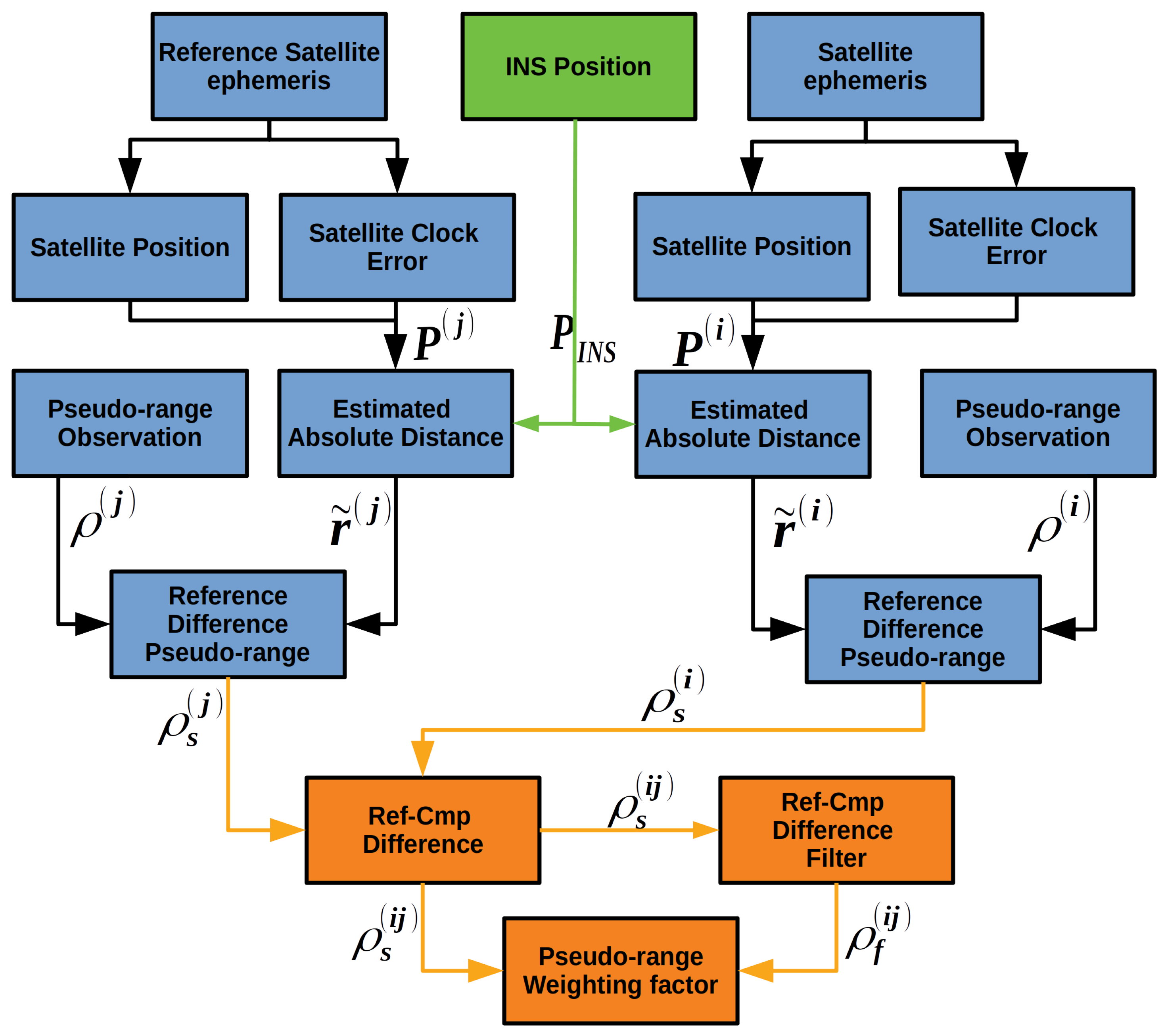
The flow diagram of IWA is shown in
Figure 6. Firstly a reference satellite is chosen from all the tracking satellites with the principle that the chosen satellite has the highest elevation angle and the strongest
. The positions and clock errors of the reference satellite and all other satellites are obtained by the ephemeris. Since the accuracy of INS is high in a short time and is not affected by environments, it can provide the vehicle position. After the compensation of lever arm, the position coordinate in Earth Centered Earth Fixed (ECEF) frame is denoted as
. With the already known satellite position coordinate
, the estimation of the absolute distance between the satellite and the vehicle can be calculated:
Then the absolute distance is deducted from pseudo-range observations:
where
is the estimation error of absolute distance. The left items in (
14) vary slowly except the receiver clock error. Next step is to eliminate the receiver clock error, which leads a difference operation between reference satellite and other satellite:
In this way, the receiver clock error is eliminated and the remain items are the ionosphere and troposphere propagation errors, which vary very slowly. The slowly varying items are then fed to a smooth filter. An
smoother will do the work.
Finally the difference between
and
is calculated:
In urban environments, if a gross error is contained in the pseudo-range observation, this error can be easily detected in this way. The
and
of a GPS satellite with PRN 5 are plotted
Figure 7. Based on the fact that under vehicle dynamics, the ionosphere and troposphere propagation errors vary slowly, the differences between the original and smoothed difference data results can reflect the errors of the pseudo-ranges. And these errors are usually caused by the signal’s blocking and reflection.
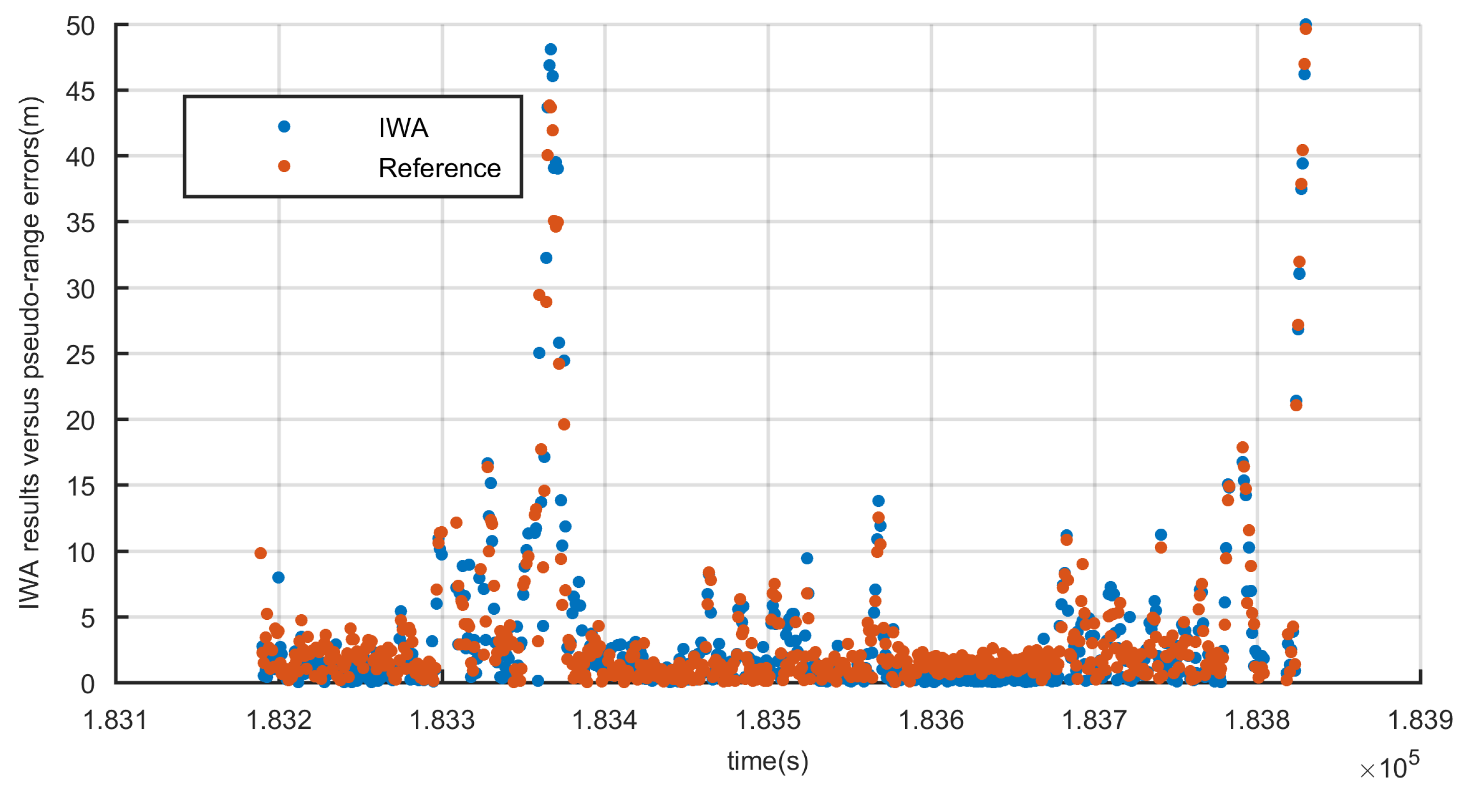
To prove above point, the IWA results
and pseudo-range errors are plotted in
Figure 8. The pseudo-range error is the difference between pseudo-range observation and reference pseudo-range. According to the high precision vehicle position provided by reference system and the position of satellite, reference pseudo-range can be calculated. The deduction of reference pseudo-range will be described in detail in
Section 4. In
Figure 8, IWA results and pseudo-range errors show high consistency. Therefore, the IWA results can correctly reflect the pseudo-range gross errors and be used to weight the pseudo-ranges, which will eliminate most of the gross errors and improve the accuracy of position greatly. In practice, the three stages weighting algorithm is applied:
where
is the weighting value of the
satellite pseudo-range observation. We set two threshold values
and
. When the estimated noise is smaller than
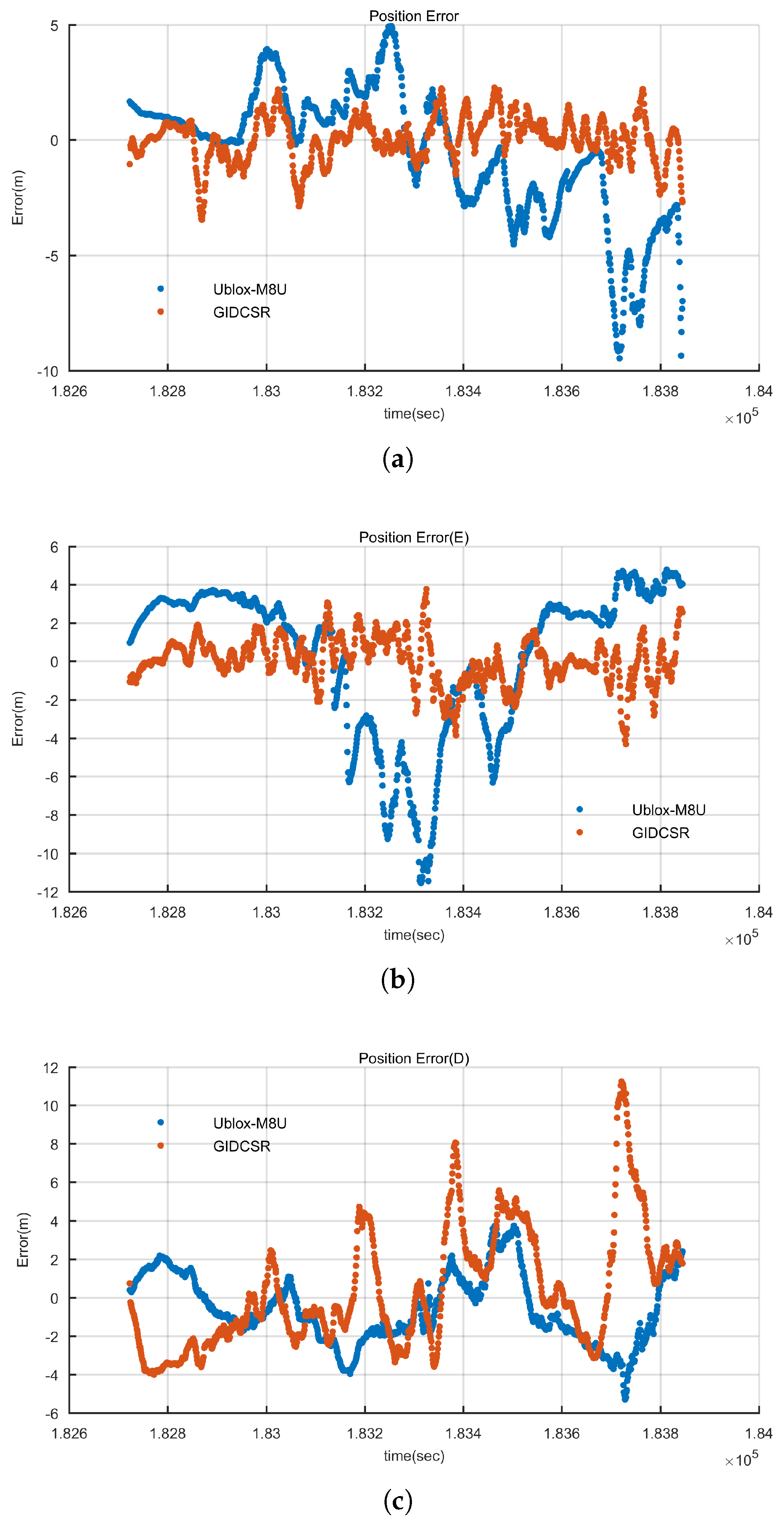
, the pseudo-range is weighted as 1. When the estimated noise is unbearable, the pseudo-range is simply thrown away. Not only can IWA improve the quality of pseudo-range, but also it can improve the accuracy of position results by weighting the pseudo-range.


