1. Introduction
Nowadays, the Digital Transformation is changing the way of understanding the different processes performed in the industrial sector. The Industry 4.0, the Internet of Things (IoT) and the Cyber-Physical Systems have arisen as the main paradigms of this digital transformation. They drive the adoption of new technologies such as data-driven based ones to support and improve the industrial processes. For instance, maintenance or control tasks can be performed automatically relying only on data provided by such a kind of data-driven systems [
1].
In that sense, one of the main tools which have arisen as one of the core concepts of the Industry 4.0 paradigm are the Artificial Neural Networks (ANNs) [
2]. They are computational models characterised by their capabilities in the modelling of highly complex and non-linear processes performed in several industries such as the chemical one [
3]. Besides, one of the most important points of ANNs is that they only need pairs of input and output measurements to model a process. This opens a wide range of processes and activities which can take advantage of these tools. For instance, predictive maintenance or detection of rare events, which are tasks giving highly-valuable information to the companies, can be performed adopting ANNs. One clear example is shown in Reference [
4], where ANNs are adopted in the petrochemical industries to automatically detect outliers such as drifts or process disturbances.
Other examples of ANNs applications are the soft-sensors, which are adopted to predict unmeasured variables by means of available data. Besides, the adoption of such sensors entail a reduction in the costs related to sensing activities [
5,
6,
7,
8,
9]. In References [
5,
6], ANNs have been considered to implement soft-sensors based on Multilayer Perceptron (MLP) structures. In both cases, the soft-sensors are placed in a refinery debutanizer column to predict the different concentrations involved in the distillation processes. In Reference [
5], the MLP has been adopted to implement a Non-linear Autoregressive model while in Reference [
6] the nets have been conceived to implement an adaptive linear based soft-sensor to predict multiple components of the distillation column. Another type of industrial processes where soft-sensors have been widely considered corresponds to the sewer systems. In Reference [
7], Long Short-Term Memory cells (LSTMs), a topology of Recurrent Neural Networks (RNNs), are considered to model the behaviour of the sewer systems and then manage them. The main idea is to forecast the amount of residual water incoming into the system and then spatially distribute it among the free space of the system.
Another field where the adoption of ANNs is continuously increasing corresponds to the wastewater treatment plants (WWTPs). They consist in industries devoted to reducing the pollutants of the residual urban waters coming from the sewer systems. To perform this, they consider highly complex and non-linear biological and biochemical processes that require some WWTP concentrations at a certain value (set-point). Besides, some control structures are applied in order to manage them. For instance, Proportional Integral (PI) controllers have been considered as the WWTP default control strategy to maintain the dissolved oxygen (
) at the fifth reactor tank and the nitrate-nitrogen (
) at the second one [
10]. On other cases, Model Predictive Controllers (MPC) and Internal Model Controllers (IMC) have been considered as more complex control strategies improving the default control ones. In Reference [
11] MPCs have been adopted to maintain the ammonium effluent concentration at the given values. IMCs are considered in Reference [
12], where this structure is proposed to implement two event-based IMC structures devoted to controlling the
and the
. The main point is that these control structures work with events instead of continuous time. Despite their good behaviour and control performance, these control strategies are based on mathematical models of the process under control and therefore, they rely on highly complex and non-linear processes. In that sense, ANNs have been considered in different works to avoid this dependence.
In some cases, ANNs are adopted to predict some measurements to feed the control strategy or to determine certain concentrations required by the control strategies. For instance, in Reference [
13], an ANN-based soft-sensor has been proposed to predict three components of the WWTP, the Chemical Oxygen Demand (COD), the Total Nitrogen (TN) and the Total Suspended Solids (TSS). In Reference [
14] a soft-sensing model with an adaptive weighted fusion is proposed to compute the quality of the water inside a WWTP. This structure is complemented with wavelet neural networks to model the non-linear WWTP process. In Reference [
15], a RNN is considered as a stage performing the predictions of the input and output data required to implement a MPC. Finally, in Reference [
16] a MLP net is proposed to model the ammonium (
) and total nitrogen (TN) of a controlled WWTP plant. The idea is to predict those moments where the WWTP is spilling effluent concentrations higher than the ones established by the local administrations. Once an exceed is detected, the control strategy devoted to reducing it actuates accordingly. Finally, in Reference [
8], LSTMs have been considered to model the complete behaviour of a WWTP and determine the effluent concentrations. Then a control strategy is applied accordingly to these values.
In terms of the control, ANNs have been considered to implement some control strategies and simplify them as well as their implementation. Some control structures are based on the use of reinforcement learning and adaptive fuzzy neural network controllers [
17,
18]. For instance, in Reference [
18], an adaptive fuzzy neural network has been considered to track the optimal set-points of the dissolved oxygen in the fifth reactor tank and the nitrate-nitrogen of the second one. Other works consider the adoption of the IMC structure due to its easy implementation and good performance [
19]. In addition, this structure is very suitable to be used as a decentralised controller since the models required by the IMC can be implemented considering ANNs over cloud-based systems while the process under control is implemented in the real plant. One example of an ANN-based IMC is shown in Reference [
20]. There, the controller is based on MLP nets in charge of tracking a variable set-point. Results show that this structure performs well in this task. In addition, it is shown that control structures based on ANNs alleviate the tedious process of designing a control structure since ANN-based models rely on data instead of highly complex mathematical models. Besides, the decoupling of the control actuation from the real processes is also achieved [
21,
22].
The common point of all these works is that they consider ideal scenarios, that is, situations where WWTP measurements are not corrupted by noise or other non-desired sensor behaviours. Nevertheless, When a real scenario is considered, the ANNs performance as well as the control one drops. To solve this, two different approaches will be proposed here. The former corresponds to the adoption of LSTM nets instead of MLPs in the IMC implementation to exploit the time correlation between measurements. The latter corresponds to a new denoising preprocessing stage which will be proposed to make the controller work with ideal and noise measurements, that is, to be able to work under ideal and real conditions. Two different Machine Learning (ML) approaches, the Principal Component Analysis (PCA) [
23] and a Denoising Autoencoder (DAE) [
24], will be consider as the denoising stage to clean the incoming measurements. In both cases, they correspond to data-driven systems which simplify the denoising stage implementation with respect to (w.r.t.) conventional solutions which involve the design of filters such as the ones considered in telecommunications receivers or in the satellite image denoising process [
25]. The adoption of these data-driven denoising techniques will improve the control metrics in the case where measurements are corrupted by noise. These measurements will be cleaned and therefore, the nets considered in the IMC implementation will be leading with ideal measurements instead of noise-corrupted ones. Furthermore, the stability analysis of the complete ANN-based IMC controller will be performed to determine the range where the IMC structure shows a robust stability.
As a summary, the contributions of this work are:
Data-driven methods have been considered to model highly complex and non-linear processes.
A new LSTM-based IMC control strategy has been designed to control the of a WWTP plant.
The stability analysis of the proposed structure is performed to determine if it is suitable to control the .
Three different ML denoising techniques will be considered to clean the noise-corrupted data entering in the LSTM-based IMC structure as well as to simplify the denoising stage implementation.
The adoption of the whole structure, (LSTM-based IMC and the denoising stage) helps in the improvement the control metrics: the Integrated Absolute Error (IAE) and the Integrated Squared Error (ISE) are improved a 21.25% and a 54.64%.
Finally, the rest of the paper is structured as follows—in
Section 2 the material and methods considered in this work are presented—the Benchmark Simulation Model No.1 (BSM1), the ANN-based IMC structure and the PCA, one of the denoising methods, are defined in this section. In
Section 3 the LSTM nets considered in the ANN-based IMC implementation and the Denoising Autoencoders considered here are described. Then, results of the different tests performed to the proposed IMC structures are shown in
Section 4. They consist in the prediction tests to determine the prediction accuracy of the considered ANNs, the stability test to determine the range of robust stability and the control test to determine the behaviour of the whole IMC structure. Finally,
Section 5 concludes the paper.
4. Results
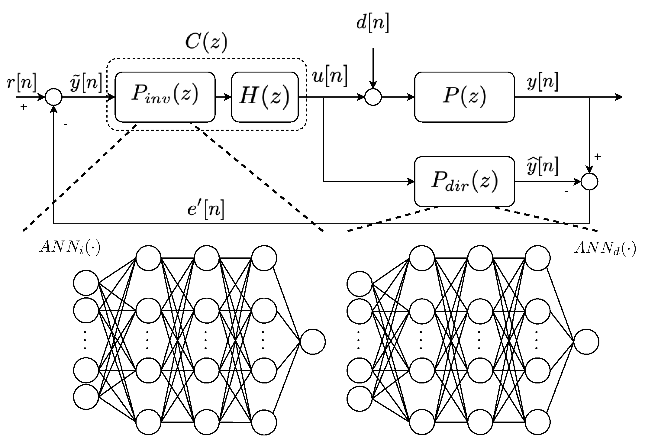
Results have been computed over the two previously mentioned scenarios: (i) the Ideal Scenario, and (ii) the Real one. In the ideal case, the default PI controlling the
concentration has been substituted by the IMC structure based on ANNs. Specially, two types of ANNs have been considered, the MLPs and the LSTMs.
and
model the direct relationships between the actuation and controlled variables.
and
model the inverse relationships of the process under control. The main point of this scenario is placed in the sensors it considers—they sense the different involved concentrations neither adding noise nor delays. This scenario has been previously analysed in Reference [
20], however, the IMC was implemented with MLP nets and its stability was not computed.
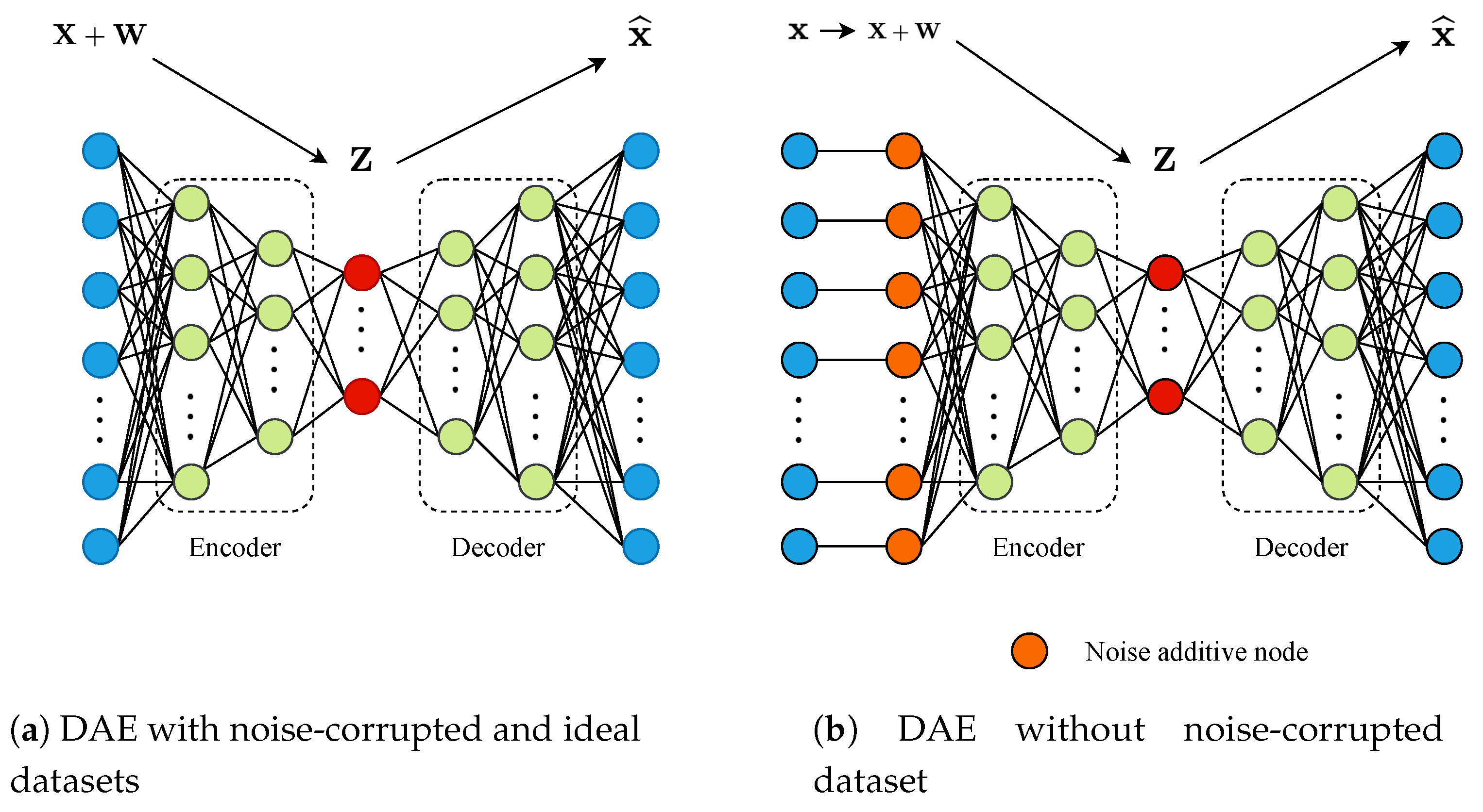
On the other hand, the real scenario considers the same IMC control strategy as in the ideal case. Nevertheless, the sensors considered here add noise and non-desired behaviours to the different measurements. Since the proposed IMC control strategy is implemented with ANNs, it highly depends on the measured data. For that reason, the controller performance drops when noise corrupted measurements are considered. To overcome this, a new denoising preprocessing stage has been proposed. It considers two different approaches, (i) the PCA and (ii) the DAE. Results will show that the DAE approach is the one offering the best behaviour when compared to the PCA.
Results of each scenario have been computed in terms of the predictions performed by the ANNs, the IMC control performance and its stability. Thereby, these results will show which are the best IMC configurations not only for the ideal scenario, but also for the real ones.
In such a context, the predictions performed by the different ANNs will be compared in terms of the Root Mean Squared Error (
), the Mean Average Percentage Error (
) and the determination coefficient (
):
where
is the mean value of the real values (labels), that is, the ones yielded by the process under control.
N corresponds to the total number of measurements.
RMSE will show the direct relationship between the predicted values and the real ones provided by the process under control, thus, the lower the metric, the lower the error. However, we are going to deal with different measurements such as the and the which are highly heterogeneous. Lets consider the , whose range corresponds to the interval day−1. The performance of the ANN predicting the aeration coefficient can show high RMSE values whereas its predictions are good enough. This is shown with MAPE. It computes the percentage of error committed in the prediction process. Consequently, this metric will complement the RMSE in the sense that it will tell if errors are large or small. Finally, is computed to show if predictions follow the tendency of the different measurements or not: the largest the , the better the predictions. RMSE and metrics have been calculated with normalised data whilst MAPE has been computed with real values to avoid divisions by 0. All the values are computed with the test dataset.
4.1. Ideal Scenario Results
4.1.1. Prediction Results
Prediction results of the Ideal Scenario are shown in
Table 1, where the RMSE, the MAPE and the
are computed for the different prediction approaches: the MLP and the LSTM nets. Autoregressive Integrated Moving Average (ARIMA) method [
55] has been also considered for comparison purposes. From these three prediction approaches, only the ANNs can be implemented in the IMC control structure: the IMC requires prediction approaches which predict the output values from the input ones (predict
from
) and vice-versa [
19]. On the other hand, the ARIMA model predicts the output measurements considering the previous observed values [
55]. In other words, ARIMA only needs
measurements to predict the
. Even thought, ARIMA results have been shown in
Table 1 to get an idea of the ANNs predictions quality. Among the different methods predicting the direct relationship, the one offering the lowest performance corresponds to the
method. This was expected since ARIMA generates its model considering only the measurements of a certain variable. Thus, the model generation process becomes a harder task than in the case where more input information is provided (MLP and LSTM nets). For instance, the
net is able to improve the RMSE and MAPE around a 71.91% and 88.47%, respectively. Then, between
and
nets, the improvement for these metrics equal to a 40% and a 77.42%, respectively. This improvement is motivated by the fact that LSTM networks take into account the dynamic evolution over the time, that is, the time-correlation between measurements. This is achieved due to the memory cell they implement and the processes they perform to the stored information ([
35], Section 10.10). In terms of the inverse models, the lowest performance is given by the
method. As observed, the ARIMA method is able to improve the MLP performance, however, it cannot be implemented in the IMC structures by the reasons stated above. Nevertheless,
overcomes not only the
results, but also the
ones. In this case, the improvement achieved by the
w.r.t. the
corresponds to a 45% in the case of the RMSE, a 25.73% in the case of the MAPE and a 1.01% in the case of the
metric. As observed, the MAPE improvement considerably differs between the direct and inverse relationships. This is directly related to the complexity of the processes being modelled, the direct process is less complex than the inverse one. Finally, the results obtained here clearly show that LSTM cells are the prediction approach offering the best performance and therefore, they are the ones considered to model the process under control.
Another point which has to be taken into account when dealing with ANNs is the overfitting problem. Although regularisation techniques can be applied to mitigate its effects, one has to analyse the results to determine if overfitting is present or not. In this case, this analysis has been performed by means of the ANNs training curves. These curves show the evolution of the ANNs cost function (Mean Squared Error—(
)) along the training process. In this case, two curves are considered: (i) the evolution of the cost function when the subset devoted to training the net is adopted (training curve) and (ii) the evolution when the subset devoted to validate the network is considered (validation curve). When overfitting is committed, there will be a point where the training curve is still decreasing towards zero whereas the validation curve starts to grow up ([
35], Chapter 7). This means that the ANN model is memorising the input/output pairs of data instead of generalising. In our case, overfitting is not committed neither in the
structures nor in the
ones since there are not any offset between training and validation curves (see
Figure 8).
4.1.2. Control Performance
Two tests are computed to determine the control performance of the proposed IMC structure. The former is focused on determining the stability of the IMC structure whereas the latter will determine the control behaviour of the whole structure. The ETFE-based method is considered here to determine which are those frequencies where the proposed IMC structure is robustly stable or not [
38,
39]. Besides, this stability test will also determine which are the most suitable cut-off frequencies (
) of the IMC low-pass filter, which is devoted to filtering non-desired behaviours related to unmodelled dynamics and inversion uncertainties of the process under control [
19].
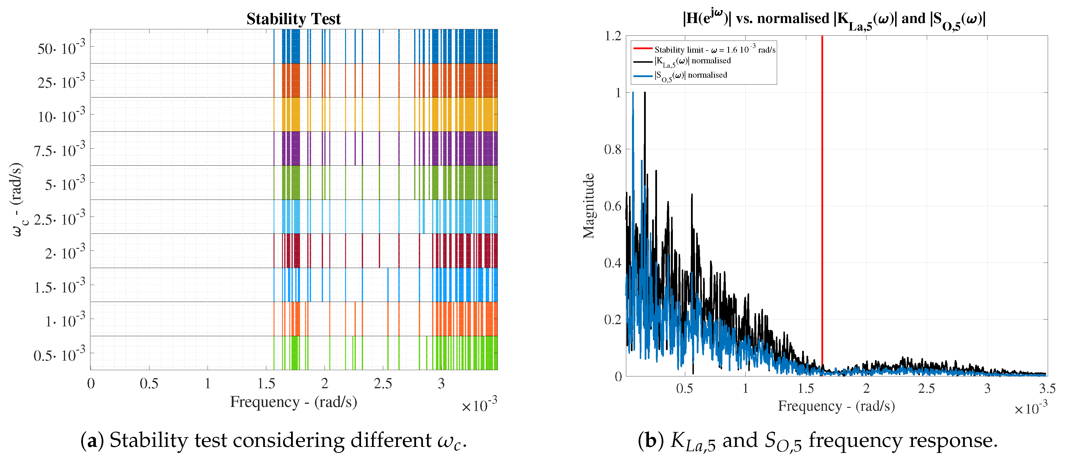
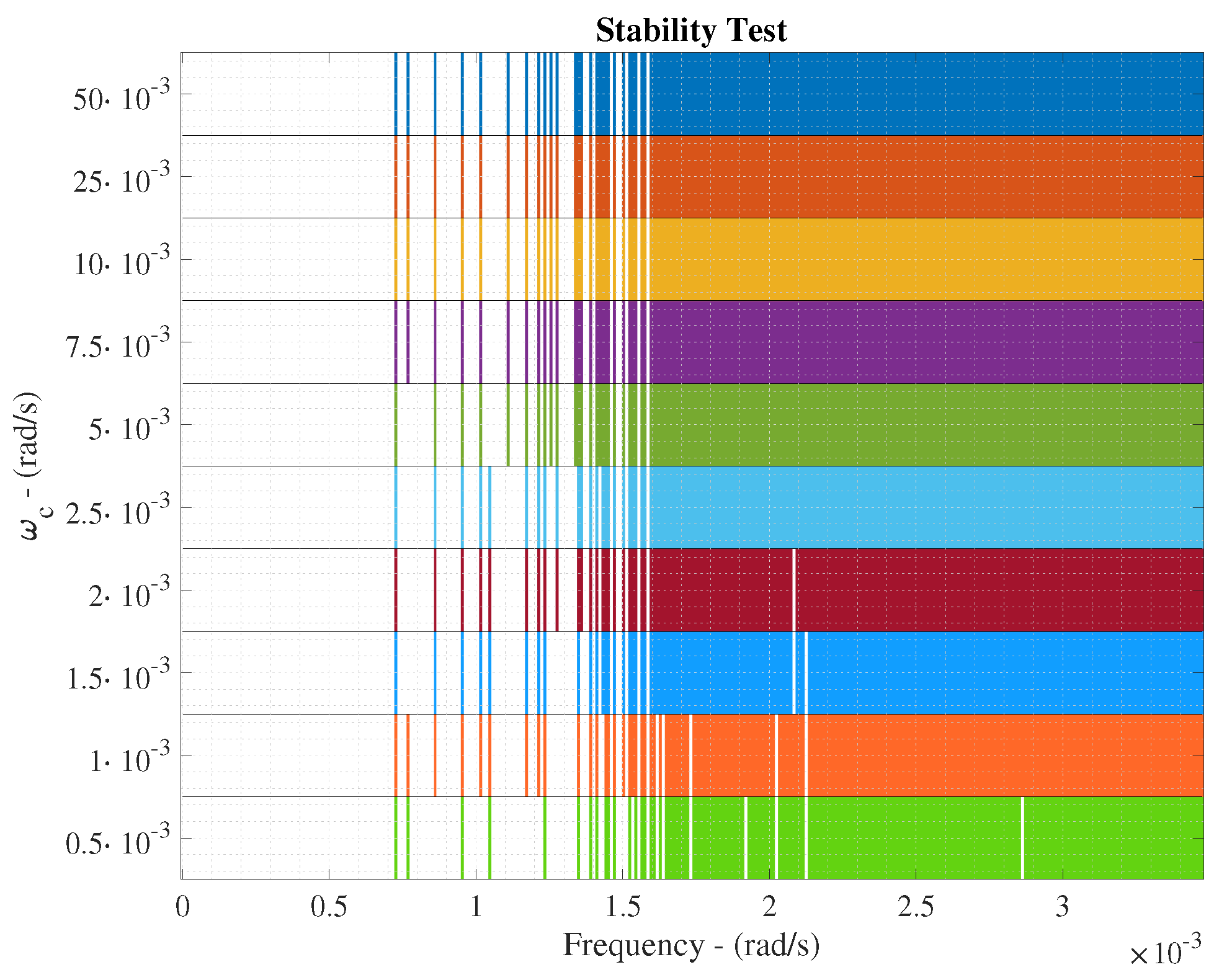
Results of the ETFE-based stability test are shown in
Figure 9a where 10 different cut-off frequencies of the IMC low-pass filter are considered. Here, those frequencies where the IMC structure stability cannot be assured are shown. For instance, if the cut-off frequency equals to
rad/s, the IMC structure is marginally stable until
rad/s. Thus, the stability of the proposed IMC approach can be assured until this frequency due to the fact that the highest frequency component of IMC input signals equals to
rad/s and it is shown by the
variable (see
Figure 9b). When the cut-off frequency is decreased, the stability range is increased, however, the filter actuation will be higher and therefore, the control performance can be degraded.
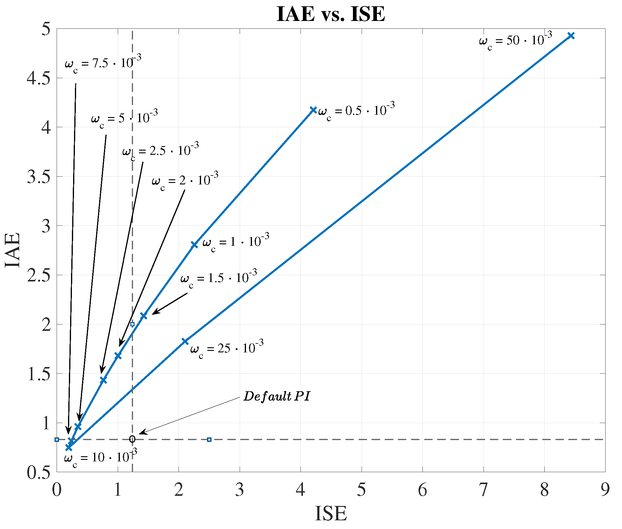
This is clearly shown in the control behaviour (see
Figure 10), where the evolution of the IAE and the ISE have been computed as a function of the cut-off frequency for a certain variable set-point (see
Figure 11). As observed,
rad/s is the optimal cut-off frequency offering the lowest values of the considered metrics:
,
. For instance, if
equals to
rad/s, a worsening in the control performance is produced—IAE and ISE are increased around a 47.76% and 73.44%, respectively.
When comparing the default PI structure with the IMC prediction approach, one can also observe that the proposed LSTM-based IMC structure is able to improve the default PI metrics: , . Thus, the highest improvement is again performed when a of rad/s is considered: the IAE and ISE metrics are improved a 39.52% and a 75.90%, respectively.
Finally, the complete structures have been tested adopting the different incoming influents: the dry, the rainy and the stormy ones. Results are shown in
Table 2, where it is observed that the proposed control is able to better track the given set-point than the default PI controller does independently of the considered weather. When rain and storm episodes are produced, the amount of influent in the WWTP increases and therefore, the oxygen concentration in the reactor tanks decreases. Moreover, if the variable set-point shows that an increment of this concentration is required, the controller will act consequently adding more oxygen in the fifth reactor tank (see
Figure 12). Then, when the LSTM-based IMC is applied, the control is better performed as shown by the IAE and ISE values.
As a summary, this LSTM-based IMC controller has been designed to track a given variational set-point independently of the influent profile entering in the WWTP plant. Results have shown that this IMC controller is able to perform the task it has been designed for better than a PI controller. For instance, the LSTM-based controller is able to improve the PI control behaviour at the expense of increasing the overall costs in some of the cases. However, this performance corresponds to an ideal scenario where neither noise nor undesired behaviours are present. If a real scenario is considered instead, the performance of the LSTM-based IMC controller drops.
4.2. Real Scenario Results
In the real scenario, real sensors are used instead of ideal ones. These are characterised by introducing different non-desired behaviours such as delays in the measurements and noise [
10]. In such a context, the IMC controller performance will drop if the LSTM nets adopted to model the process under control in the ideal scenario are not modified accordingly to the new circumstances (see
Table 3). For instance, their IAE and ISE metrics are now around 1.90 and 0.83, respectively, which represents an average increment in the IAE and ISE around a 63.16% and a 79.52% w.r.t the ideal scenario. Besides, if we compute the difference of the improvements between the ideal and the real scenario, we will observe that the IAE and ISE improvements have been degraded around a 30.49 and 34.83 percentage points, respectively. This change is motivated by the design of the PI and the IMC controller. Although the PI showed a good performance in the ideal scenario, it has not been conceived to deal with real measurements [
10]. For that reason, the LSTM-based IMC is able to improve the control behaviour. Moreover, they can be improved even more if actions to mitigate the loss of improvement are considered.
4.2.1. Prediction Performance
The first prediction approach consists in retraining the ANNs to model the process under control considering the effects of noise. In that manner, the ANNs will perform predictions of ideal measurements from noisy ones. Results of this approach are shown in
Table 4, where the prediction metrics have been computed once the training process has ended. In addition, the ARIMA performance has been considered again as a baseline although it cannot be implemented in an IMC structure. In this case, the performance of
, the model in charge of the direct relationship, has been degraded until it shows an
three times bigger than in the ideal case (
), a
equal to 282.09% and a
of
. Results of the
clearly show that ARIMA models cannot be considered not only by the aforementioned fact, but also by generating a model not able to deal with noisy signals. It is worth mentioning that
, the model in charge of forecasting the actuation variable (
), is exactly equal to the ideal case. This is motivated by the fact that the actuation variable is not corrupted by noise since it is a value computed by the IMC. Moreover, it actuates directly over the oxygen valve without going through a sensor but through an actuator which adds a delay [
10].
MLP and LSTM results show that the prediction performance is degraded w.r.t. the ideal scenario. This effect is expected since the nets have to model the process under control taking into account measurements corrupted by noise. For instance, the
has increased from 0.030 to 0.043 and from 0.045 to 0.101 in the
and
nets, respectively. This is translated into a degradation between a 30.23% and a 55.44%. If the performance is only compared in terms of the noise scenario, we will observe that the improvement of LSTMs w.r.t. the MLP equals to a 62.55% and a 58.48% in average for the
and
values, respectively. Analysing the last ones, one will observe that they equal to a 15.85% and a 36.90% for the
and the
, respectively. This shows that training the neural networks with noisy signals will entail the appearance of high errors and therefore, an incorrect control behaviour. Moreover, these errors can destabilise the whole system as it is shown in
Figure 13, where the robust stability of the whole system cannot be assured for frequencies higher than
rad/s.
In such a context, the denoising stage solutions are proposed with a twofold objective—(i) increase the range where the whole IMC controller is marginally stable and (ii) improve the control behaviour of the whole system. Thus, the performance of this stage will be computed in terms of the denoising accuracy, the stability of the considered denoising approaches and finally the control performance.
The accuracy results are shown in
Table 5, where the
, the
and the
metrics are computed for the PCA-based, the MLP-based and the LSTM-based denoising approaches. As it is observed, the structure offering the best performance is the MLP-SW, which corresponds to the MLP-based DAE implemented with a SW of 4 h. In this case, the accuracy metrics show that this structure is able to offer a
equal to 0.089, a
around a 3.72% and a determination coefficient of 0.99. Besides, there are other approaches showing a good denoising accuracy. For instance, the LSTM-based DAE and the PCA-SW approaches are offering
values equal to 0.091 and 0.131, respectively. In percentage, these values correspond to a worsening of 2.20% and 32.06% w.r.t. the MLP-SW approach. In terms of the
and
, the worsening between the LSTM-SW and the PCA-SW w.r.t the MLP-SW is around 3.2 and 5.6 percentage points for the
and 0.01 units for the
. This shows that among the different structures these three are the ones which can be considered as a denoising tool.
Let us suppose that a real sensor has measured a
concentration equal to
mg/L (real measurement + noise). However, the ideal measurement, that is, without noise, corresponds to
mg/L. To overcome this measurement error, a denoising approach is considered. When applying a simple MLP, the new value will be in the range
–
due to the fact that its
equals to
. On the other hand, the denoised measurement will be placed in the range
–
when a MLP-SW approach is adopted. Consequently, the lower the
values, the better the denoising approach. For that reason, those approaches showing high
(over 10%) have been directly neglected. The denoising process carried out by the different denosing approaches can be observed in
Figure 14, where the noisy, the ideal and denoised
signals are shown for the PCA-SW, MLP-SW and LSTM-SW approaches. Their denoising performance is shown in
Table 5.
4.2.2. Control Performance
Before computing the control performance, the stability of the system has to be analysed. The ETFE-based analysis has shown that none of the different denoising approaches are able to assure a robust stability below the
rad/s, however, they are able to increase the stability margin w.r.t. the LSTM-based nets retrained with noisy signals (see
Figure 15). For instance, the retrained LSTM-based nets are able to increase the bandwidth where the controller is able to work from the
rad/s until at least the
rad/s (when a
rad/s is chosen). Although this frequency is lower than the stability limit of the ideal case, it is worth to notice that the MLP-SW approach is able to offer a greater margin of stability (until the
rad/s) at the same time it only fails the ETFE-based stability test in three frequencies below the
rad/s. Neither the LSTM-SW nor the PCA-SW are able to pass the stability test in more frequencies than the MLP-SW does. For that reason, the
-
approach is the best candidate to be adopted as the principal denoising approach. This will also be confirmed analysing the control behaviour. In such a context, the same
as in the ideal scenario will be considered since the LSTM-based IMC controller is the same.
The control performance of the LSTM-based IMC considering a denoising process has been computed adopting the three most suitable approaches (PCA-SW, MLP-SW and LSTM-SW). The prediction part of this LSTM-based IMC structure corresponds to the LSTM cells considered in the ideal scenario. Therefore, any improvement w.r.t. the results shown in
Table 3 will be directly related to the behaviour of the denoising approaches. In that sense, results of the whole system are shown in
Table 6. The IAE and ISE metrics show that the control strategy is yielding better results than the default PI. This is directly related to the noise effect: the denoising approaches are filtering the noise of the signals entering in the
and
nets. However, the
and the
coming from the real plant are noise-corrupted. As a consequence, the mismatch between the real
and the predicted one will contain noise components. Moreover, DAEs are denoising approaches with losses able to reduce the noise of the signals at expense of recovering them with small variations. Consequently, although denoising techniques have been considered, part of the noise effect is still present in the predictions performed by
and
. These will entail the generation of
values which differs from the ones required to track the
in the best way. Even though, if no denoising stage is considered, the tracking process is worst performed as shown in
Table 3.
Analysing the numerical results, it is observed that the best improvement w.r.t. the default PI structure is offered by the MLP-SW approach. It achieves an average improvement around a 21.25% for the IAE and a 54.64% for the ISE, while the PCA-SW and the LSTM-SW approaches achieve lower values of the IAE and ISE metrics. These results show that the three considered approaches are valid as a denoising stage previous to the LSTM-based IMC control structure. Not only this, the stability of the control structure has to also be taken into account. As shown in
Figure 9a, the MLP-SW is again the denoising approach offering the higher stability margin. Besides, if the controlled signals are compared, we will observe that the MLP-SW approach is the one offering the most accurate signal, that is, the MLP-SW approach is the one performing the best tracking process (see
Figure 16). On the other hand, the LSTM-SW approach shows some points where the tracking process differs even more than the PI approach. This fact motivates the adoption of the MLP-SW denoising approach as the main denoising tool and the LSTM-based IMC as the main control structure.
5. Conclusions
In this work a new IMC control strategy and a denoising preprocessing stage have been proposed. They have been deployed and implemented over a WWTP where the main objective is to control the dissolved oxygen concentration in the fifth reactor tank. One of the points of this new control approach is placed in the direct and inverse models of the process under control. ANNs have been considered to generate these models instead of generating them as it is done in conventional processes. Since this work is focused on WWTPs, the different measurements (concentrations) can be conceived as time-series showing a high correlation in time. As a consequence, LSTM nets have been proposed in the direct and inverse model generation process due to their ability in modelling highly complex and non-linear processes as well as time-series signals. This approach has been tested over BSM1 framework when ideal sensors are adopted. Results have shown that the proposed LSTM-based IMC is able to improve the default BSM1 PI control strategy metrics, the IAE and ISE, around a 43.28% and a 79.12% in average, respectively. Moreover, an ETFE-based stability test is performed to determine the controller robust stability margin. However, this situation changes when real sensors adding noise and delays to the measurements are adopted. A degradation of the control is performed if no action is proposed to overcome the noise problem.
Two different approaches can be adopted in such a situation, the retraining of the LSTM nets or the adoption of a denoising stage. The former option is simple, it only requires a retraining of the nets adopting noisy measurements instead of ideal ones. In this case, results show that LSTM nets are able to improve the RMSE a 59.81% and a 88.50% when compared with the MLP and the ARIMA approaches modelling the direct relationship between the actuation and control signals. Nevertheless, this entails a degradation of the stability, which cannot be assured for the frequency range of the control input signals. This has been solved considering the denoising stage. Two different approaches have been considered, a PCA solution and the application of DAEs. Among the different DAEs, two different configurations have been considered, the application of MLP and LSTM nets. In addition, both approaches have been tested and implemented considering the adoption of a sliding window of 4 h of WWTP concentrations. In such a context, the denoising accuracy shows that the best denoising approach is offered by the MLP-SW which shows a RMSE, a MAPE and a equal to 0.089, 3.72% and 0.99, respectively. Besides, once implemented as a control strategy, results show that the IAE and ISE metrics have been improved w.r.t. the default PI in a 21.25% and a 54.64%, respectively. The robust stability margin has been increased until the point where the whole control structure is robustly stable for nearly all the working frequencies. Only three frequencies in the range between the rad/s and the rad/s can compromise the stability.
In this context, the main goal of this new control and denoising approach is not only placed in its performance, but also in its implementation. The LSTM-based IMC as well as the DAE correspond to data-driven approaches which only require pairs of input/output data of the process under control. This entail that they can be applied to control any industrial process as long as data from the process to be controlled are available. Besides, the fact of being based on data motivates the adoption of these approaches as decentralised cloud-based control structures, where the control is performed remotely as a cloud-based service. In addition, another goal of these approaches is that they entail a reduction of the complexity in the control structure design process since the design of denoising filters or the computation of mathematical models are not required.


