Fast Single-Image HDR Tone-Mapping by Avoiding Base Layer Extraction


Abstract
:1. Introduction
- Our approach obtains tone-mapped HDR images with the help of contrast enhancement, making it unnecessary to perform any smoothing operations.
- The proposed approach tries to approximate the exposure information of the input HDR image faithfully. This information aids contrast enhancement so that our method does not require any post-processing.
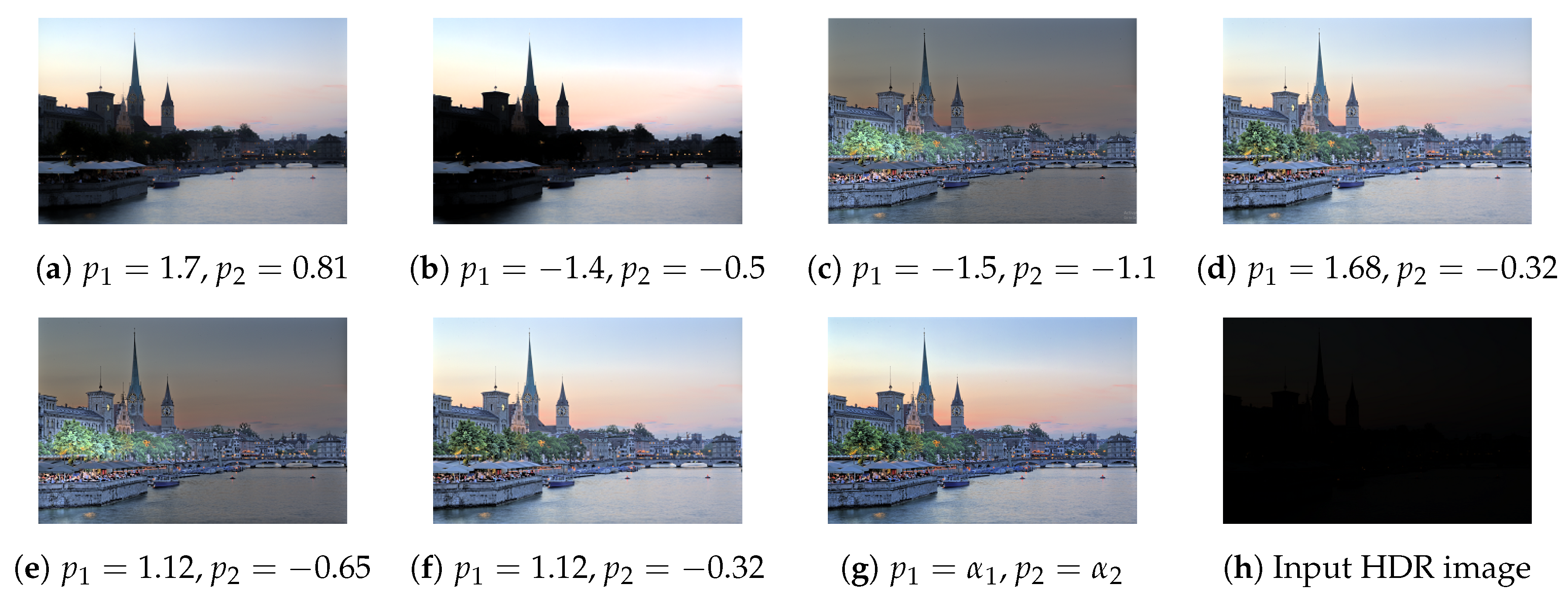
- The proposed adaptive parameter selection improves the holistic contrast correction performance.
- Our utilized weight matrix extraction scheme [2] improves the overall contrast optimization performance.
- Since this approach does not involve a smoothing operation or detail enhancement, tone-mapped images do not exhibit ringing effect or halo effect. Additionally, it is computationally faster than other state-of-the-art methods due to its single-channel contrast optimization step.
2. Related Work
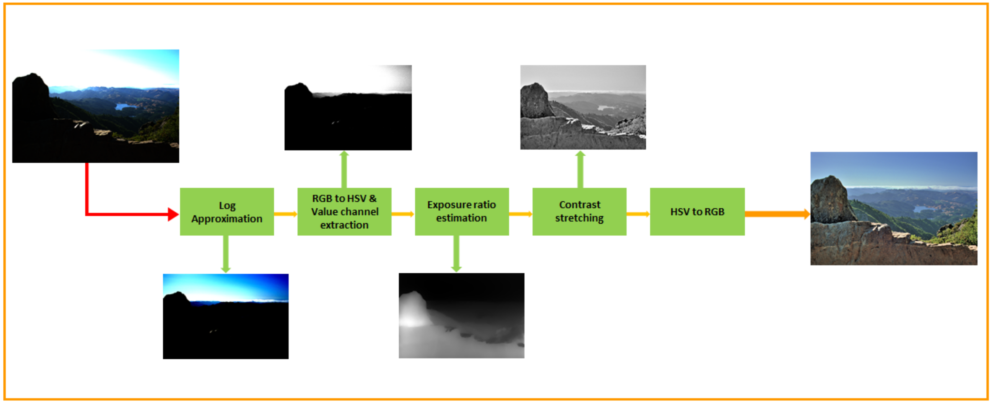
3. Methodology
4. Comparative Analysis
4.1. Dataset
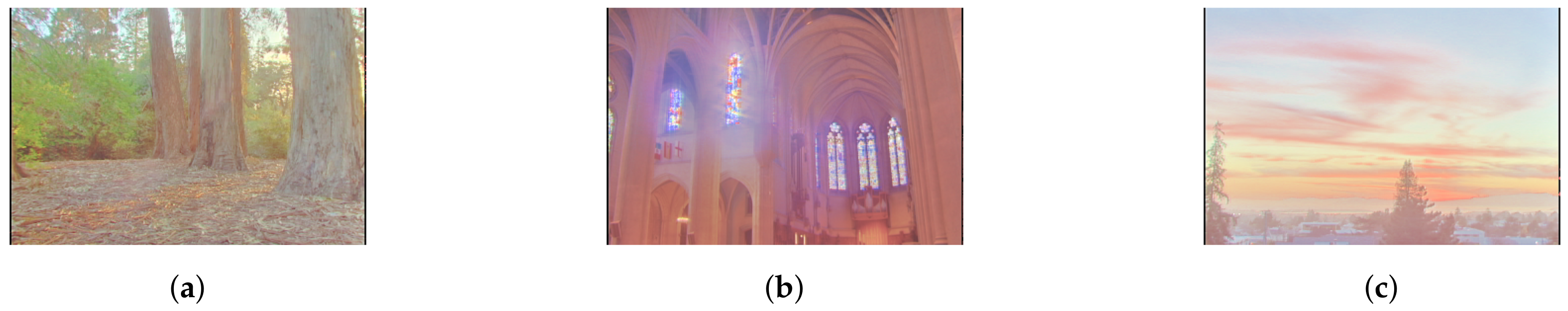
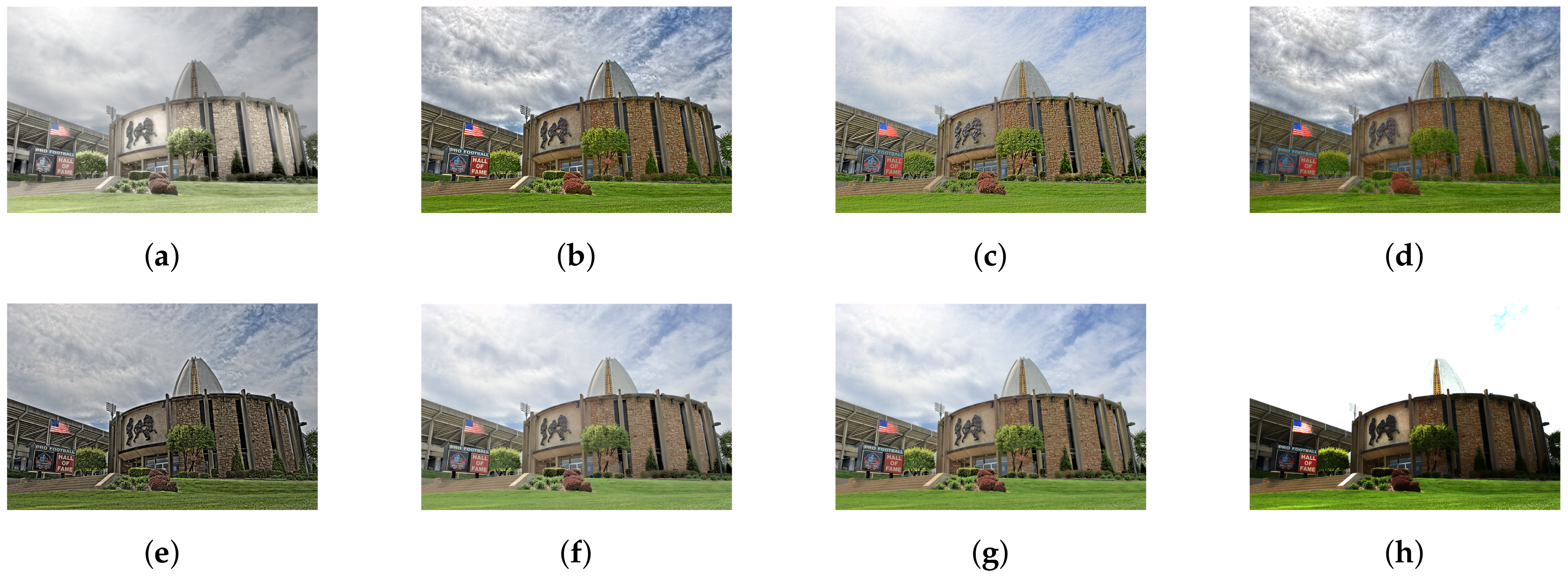
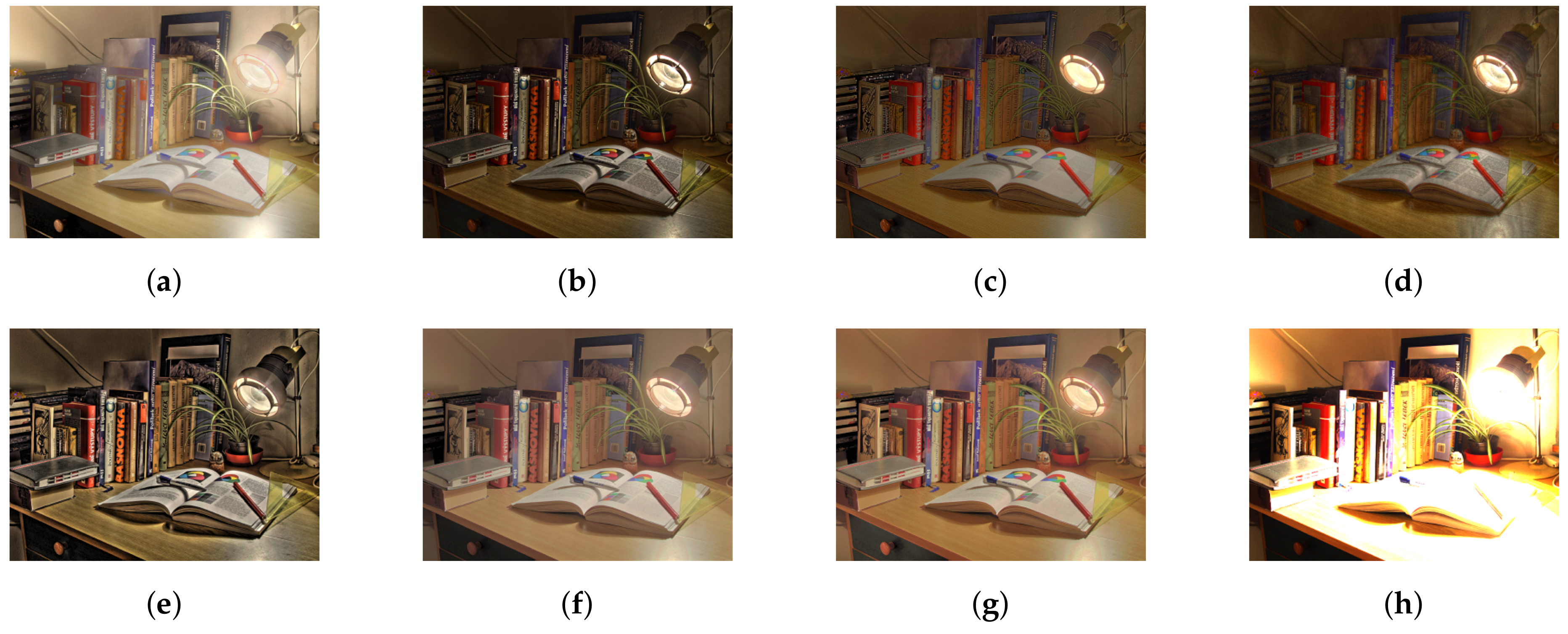
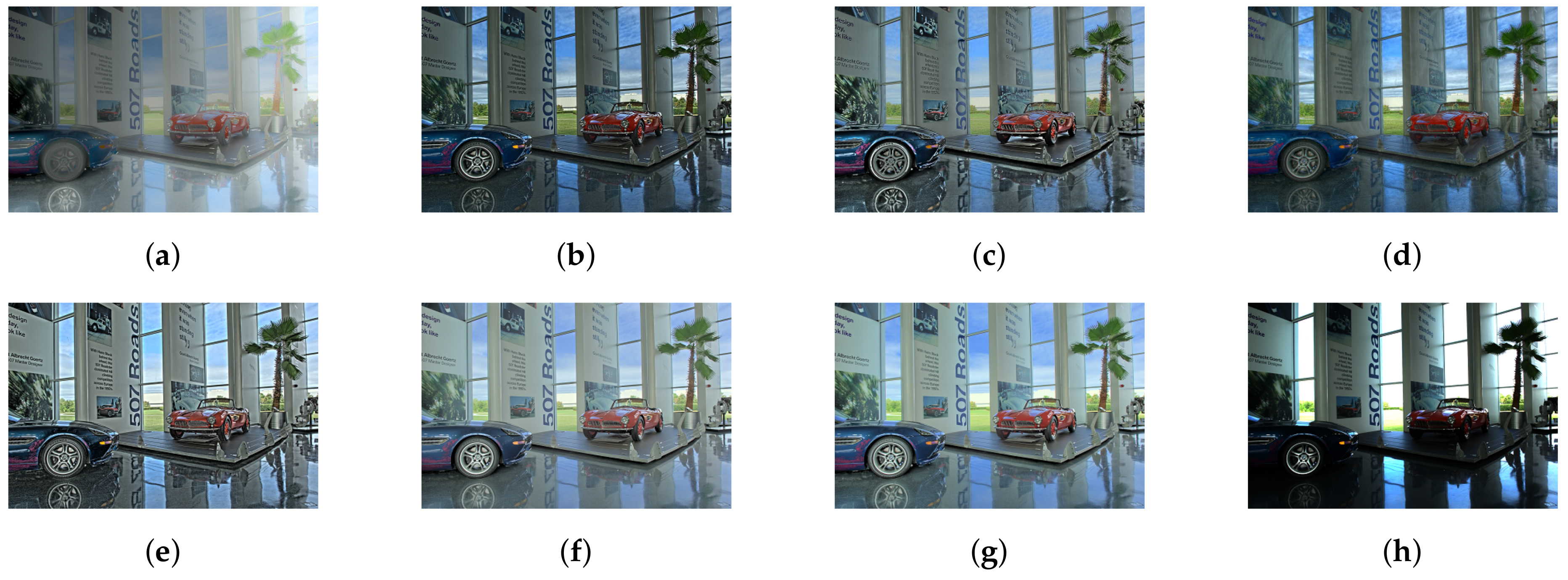
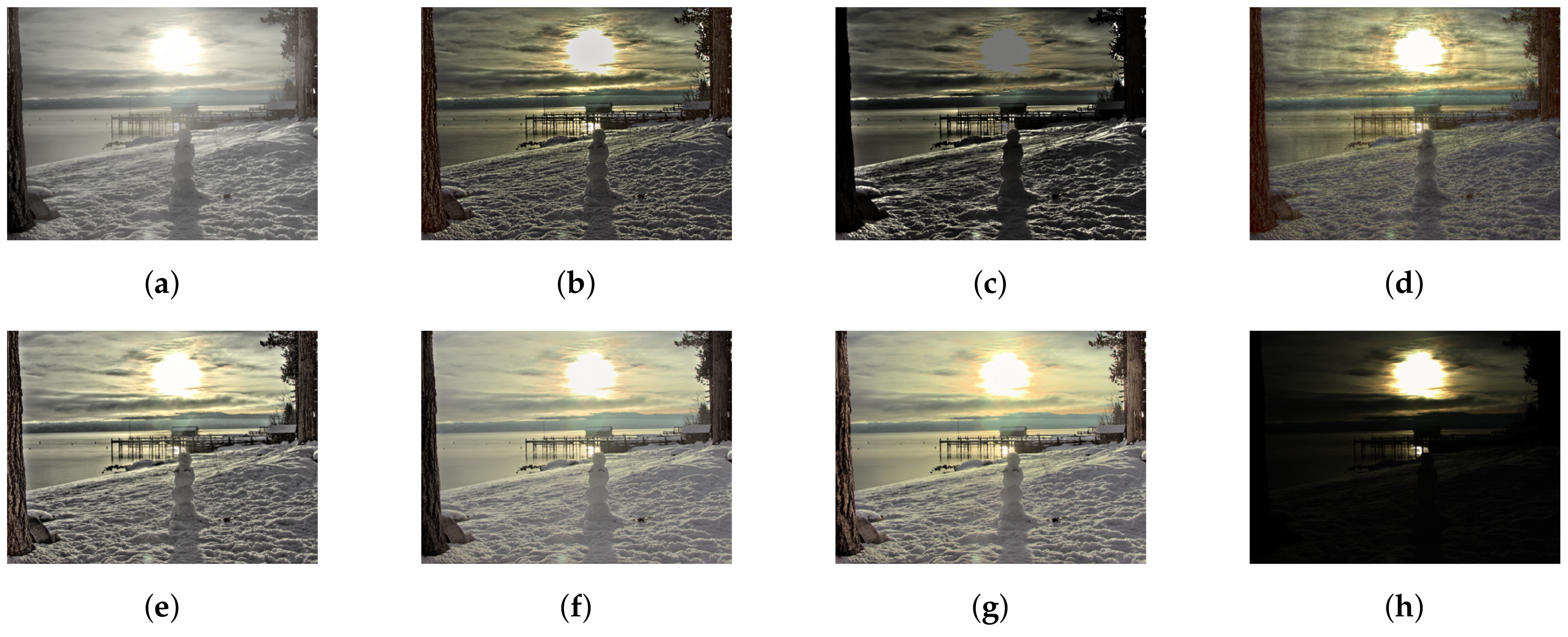
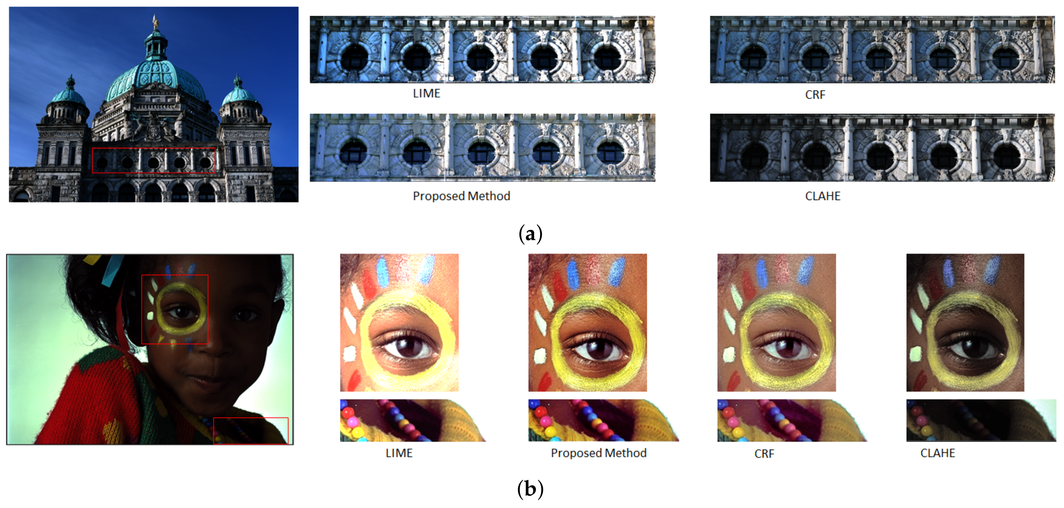
4.2. Visual Analysis
4.3. Subjective Analysis
4.4. TMQI Analysis
4.5. Time Analysis
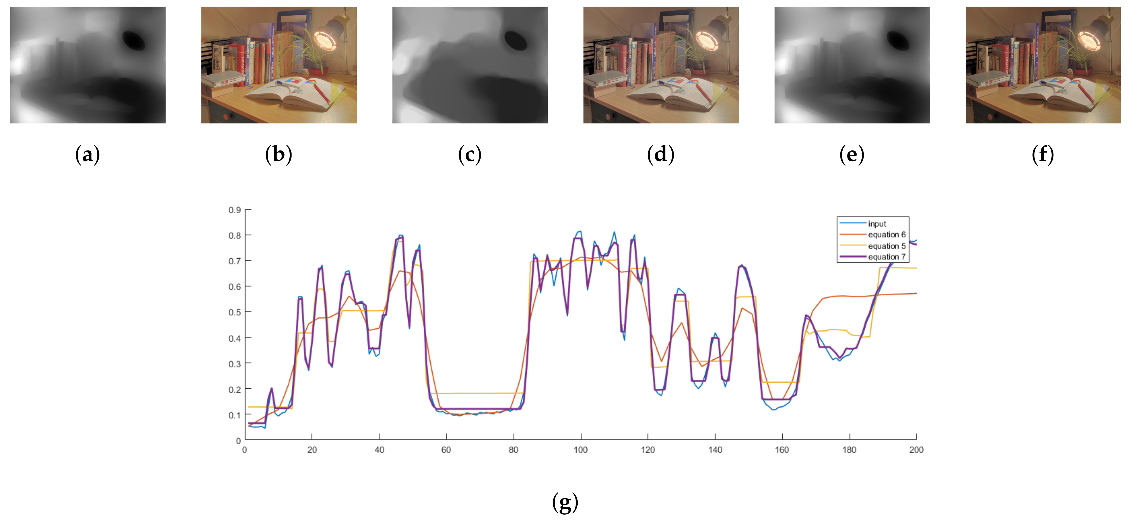
4.6. Contrast Correction Analysis
5. Conclusions
Author Contributions
Funding
Conflicts of Interest
References
- Shibata, T.; Tanaka, M.; Okutomi, M. Gradient-domain image reconstruction framework with intensity-range and base-structure constraints. In Proceedings of the IEEE Conference on Computer Vision and Pattern Recognition, Las Vegas, NV, USA, 26 June–1 July 2016; pp. 2745–2753. [Google Scholar]
- Cai, B.; Xing, X.; Xu, X. Edge/structure preserving smoothing via relativity-of-Gaussian. In Proceedings of the 2017 IEEE International Conference on Image Processing (ICIP), Fez, Morocco, 22–24 May 2017; pp. 250–254. [Google Scholar]
- Drago, F.; Myszkowski, K.; Annen, T.; Chiba, N. Adaptive logarithmic mapping for displaying high contrast scenes. Comput. Graph. Forum. 2003, 22, 419–426. [Google Scholar] [CrossRef]
- Tumblin, J.; Rushmeier, H. Tone reproduction for realistic images. IEEE Comput. Graphics Appl. 1993, 13, 42–48. [Google Scholar] [CrossRef]
- Ward, G.J. The radiance lighting simulation and rendering system. In Proceedings of the 21st Annual Conference on Computer Graphics and Interactive Techniques, Orlando, FL, USA, 24–29 July 1994; pp. 459–472. [Google Scholar]
- Li, H.; Jia, X.; Zhang, L. Clustering based content and color adaptive tone mapping. Comput. Vis. Image Underst. 2018, 168, 37–49. [Google Scholar] [CrossRef]
- Reinhard, E.; Devlin, K. Dynamic range reduction inspired by photoreceptor physiology. IEEE Trans. Visual Comput. Graph. 2005, 11, 13–24. [Google Scholar] [CrossRef]
- Ma, K.; Yeganeh, H.; Zeng, K.; Wang, Z. High dynamic range image compression by optimizing tone mapped image quality index. IEEE Trans. Image Process. 2015, 24, 3086–3097. [Google Scholar]
- Yeganeh, H.; Wang, Z. Objective quality assessment of tone-mapped images. IEEE Trans. Image Process. 2012, 22, 657–667. [Google Scholar] [CrossRef]
- Duan, J.; Bressan, M.; Dance, C.; Qiu, G. Tone-mapping high dynamic range images by novel histogram adjustment. Pattern Recognit. 2010, 43, 1847–1862. [Google Scholar] [CrossRef]
- Ferradans, S.; Bertalmio, M.; Provenzi, E.; Caselles, V. An analysis of visual adaptation and contrast perception for tone mapping. IEEE Trans. Pattern Anal. Mach. Intell. 2011, 33, 2002–2012. [Google Scholar] [CrossRef] [Green Version]
- Shan, Q.; Jia, J.; Brown, M.S. Globally optimized linear windowed tone mapping. Pattern Recognit. 2009, 16, 663–675. [Google Scholar]
- Li, Y.; Sharan, L.; Adelson, E.H. Compressing and companding high dynamic range images with subband architectures. ACM Trans. Graph. 2005, 24, 836–844. [Google Scholar] [CrossRef] [Green Version]
- Gu, H.; Wang, Y.; Xiang, S.; Meng, G.; Pan, C. Image guided tone mapping with locally nonlinear model. In Proceedings of the European Conference on Computer Vision, Florence, Italy, 7–13 October 2012; Springer: Berlin/Heidelbeg, Germany, 2012; pp. 786–799. [Google Scholar]
- Chen, H.T.; Liu, T.L.; Fuh, C.S. Tone reproduction: A perspective from luminance-driven perceptual grouping. Int. J. Comput. Vis. 2005, 65, 73–96. [Google Scholar] [CrossRef]
- Fattal, R.; Lischinski, D.; Werman, M. Gradient domain high dynamic range compression. ACM Trans. Graph. 2002, 21, 249–256. [Google Scholar] [CrossRef] [Green Version]
- Fattal, R. Edge-avoiding wavelets and their applications. ACM Trans. Graph. 2009, 28, 1–10. [Google Scholar]
- Raskar, R.; Ilie, A.; Yu, J. Image Fusion for Context Enhancement and Video Surrealism; ACM SIGGRAPH: New York, NY, USA, 2005. [Google Scholar]
- Connah, D.; Drew, M.S.; Finlayson, G.D. Spectral edge image fusion: Theory and applications. In Proceedings of the European Conference on Computer Vision, Zurich, Switzerland, 6–12 September 2014; Springer: Cham, Switzerland, 2014; pp. 65–80. [Google Scholar]
- Wu, S.; Yang, L.; Xu, W.; Zheng, J.; Li, Z.; Fang, Z. A mutual local-ternary-pattern based method for aligning differently exposed images. Comput. Vis. Image Underst. 2016, 152, 67–78. [Google Scholar] [CrossRef]
- Sun, J.; Zhu, H.; Xu, Z.; Han, C. Poisson image fusion based on Markov random field fusion model. Inf. Fusion 2013, 14, 241–254. [Google Scholar] [CrossRef]
- Durand, F.; Dorsey, J. Fast bilateral filtering for the display of high-dynamic-range images. ACM Trans. Graph. 2002, 21, 257–266. [Google Scholar] [CrossRef] [Green Version]
- Gu, B.; Li, W.; Zhu, M.; Wang, M. Local edge-preserving multi-scale decomposition for high dynamic range image tone mapping. IEEE Trans. Image Process. 2012, 22, 70–79. [Google Scholar]
- Meylan, L.; Susstrunk, S. High dynamic range image rendering with a retinex-based adaptive filter. IEEE Trans. Image Process. 2006, 15, 2820–2830. [Google Scholar] [CrossRef] [Green Version]
- Mai, Z.; Mansour, H.; Mantiuk, R.; Nasiopoulos, P.; Ward, R.; Heidrich, W. Optimizing a tone curve for backward-compatible high dynamic range image and video compression. IEEE Trans. Image Process. 2010, 20, 1558–1571. [Google Scholar]
- Barakat, N.; Hone, A.N.; Darcie, T.E. Minimal-bracketing sets for high-dynamic-range image capture. IEEE Trans. Image Process. 2008, 17, 1864–1875. [Google Scholar] [CrossRef]
- Debevec, P.E.; Malik, J. Recovering high dynamic range radiance maps from photographs. ACM SIGGRAPH 2008, 31, 1–10. [Google Scholar]
- Farbman, Z.; Fattal, R.; Lischinski, D.; Szeliski, R. Edge-preserving decompositions for multi-scale tone and detail manipulation. ACM Trans. Graph. 2008, 27, 1–10. [Google Scholar] [CrossRef]
- Liang, Z.; Xu, J.; Zhang, D.; Cao, Z.; Zhang, L. A Hybrid l1-l0 Layer Decomposition Model for Tone Mapping. In Proceedings of the IEEE conference on computer vision and pattern recognition 2018, Salt Lake City, UT, USA, 18–22 June 2018; pp. 4758–4766. [Google Scholar]
- Choudhury, A.; Medioni, G. Hierarchy of nonlocal means for preferred automatic sharpness enhancement and tone mapping. JOSA A 2013, 30, 353–366. [Google Scholar] [CrossRef] [PubMed] [Green Version]
- Paris, S.; Hasinoff, S.W.; Kautz, J. Local laplacian filters: Edge-aware image processing with a laplacian pyramid. ACM Trans. Graph. 2011, 30, 68. [Google Scholar] [CrossRef]
- Endo, Y.; Kanamori, Y.; Mitani, J. Deep reverse tone mapping. ACM Trans. Graph. 2017, 36, 1–10. [Google Scholar] [CrossRef]
- Eilertsen, G.; Kronander, J.; Denes, G.; Mantiuk, R.K.; Unger, J. HDR image reconstruction from a single exposure using deep CNNs. ACM Trans. Graph. 2017, 36, 1–15. [Google Scholar] [CrossRef]
- Marnerides, D.; Bashford-Rogers, T.; Hatchett, J.; Debattista, K. ExpandNet: A deep convolutional neural network for high dynamic range expansion from low dynamic range content. Comput. Graph. Forum 2018, 37, 37–49. [Google Scholar] [CrossRef] [Green Version]
- Kinoshita, Y.; Kiya, H. iTM-Net: Deep Inverse Tone Mapping Using Novel Loss Function Considering Tone Mapping Operator. IEEE Access 2019, 7, 73555–73563. [Google Scholar] [CrossRef]
- Ying, Z.; Li, G.; Ren, Y.; Wang, R.; Wang, W. A new low-light image enhancement algorithm using camera response model. In Proceedings of the IEEE International Conference on Computer Vision Workshops 2017, Venice, Italy, 22–29 October 2017; pp. 3015–3022. [Google Scholar]
- Chen, S.D.; Ramli, A.R. Contrast enhancement using recursive mean-separate histogram equalization for scalable brightness preservation. IEEE Trans. Consum. Electron. 2003, 49, 1301–1309. [Google Scholar] [CrossRef]
- Sen, D.; Pal, S.K. Automatic exact histogram specification for contrast enhancement and visual system based quantitative evaluation. IEEE Trans. Image Process. 2010, 20, 1211–1220. [Google Scholar] [CrossRef] [Green Version]
- Vonikakis, V.; Andreadis, I.O.; Gasteratos, A. Fast centre–surround contrast modification. IET Image Process. 2008, 2, 19–34. [Google Scholar] [CrossRef]
- Wang, L.; Xiao, L.; Liu, H.; Wei, Z. Variational Bayesian method for retinex. IEEE Trans. Image Process. 2014, 23, 3381–3396. [Google Scholar] [CrossRef] [PubMed]
- Beghdadi, A.; Le Negrate, A. Contrast enhancement technique based on local detection of edges. Comput. Vis. Graph. Image Process. 1989, 46, 162–174. [Google Scholar] [CrossRef]
- Gonzales, R.C.; Woods, R.E. Digital Image Process; Prentice Hall Press: Upper Saddle River, NJ, USA, 2002. [Google Scholar]
- Baxes, G.A. Digital Image Processing: Principles and Applications; Weily Press: Hoboken, NJ, USA, 1994. [Google Scholar]
- Kwon, H.-J.; Lee, S.-H. Contrast Sensitivity Based Multiscale Base–Detail Separation for Enhanced HDR Imaging. Appl. Sci. 2020, 10, 2513. [Google Scholar] [CrossRef] [Green Version]
- Liu, Y.; Lv, B.; Huang, W.; Jin, B.; Li, C. Anti-Shake HDR Imaging Using RAW Image Data. Information 2020, 11, 213. [Google Scholar] [CrossRef] [Green Version]
- Choi, H.-H.; Kang, H.-S.; Yun, B.-J. Tone Mapping of High Dynamic Range Images Combining Co-Occurrence Histogram and Visual Salience Detection. Appl. Sci. 2019, 9, 4658. [Google Scholar] [CrossRef] [Green Version]
- Rousselot, M.; Le Meur, O.; Cozot, R.; Ducloux, X. Quality Assessment of HDR/WCG Images Using HDR Uniform Color Spaces. J. Imaging 2019, 5, 18. [Google Scholar] [CrossRef] [Green Version]
- Khan, I.R.; Rahardja, S.; Khan, M.M.; Movania, M.M.; Abed, F. A Tone-Mapping Technique Based on Histogram Using a Sensitivity Model of the Human Visual System. IEEE Trans. Ind. Electr. 2018, 65, 3469–3479. [Google Scholar] [CrossRef]
- Guo, X.; Li, Y.; Ling, H. LIME: Low-light image enhancement via illumination map estimation. IEEE Trans. Image Process. 2016, 26, 982–993. [Google Scholar] [CrossRef]
- Xu, L.; Lu, C.; Xu, Y.; Jia, J. Image smoothing via L0 gradient minimization. In Proceedings of the SIGGRAPH Asia Conference 2011, Hong Kong, China, 12–15 December 2011; pp. 1–12. [Google Scholar]
- Reza, A.M. Realization of the contrast limited adaptive histogram equalization (CLAHE) for real-time image enhancement. J. VLSI Signal Proc. Syst. 2004, 38, 35–44. [Google Scholar] [CrossRef]
- Xiao, B.; Xu, Y.; Tang, H.; Bi, X.; Li, W. Histogram Learning in Image Contrast Enhancement. In Proceedings of the IEEE Conference on Computer Vision and Pattern Recognition Workshops 2019, Long Beach, CA, USA, 16–20 June 2019. [Google Scholar]


| Methods | Mean | Standard Deviation |
|---|---|---|
| LW [12] | 3.46 | 0.23 |
| WLS [28] | 4.1 | 0.19 |
| RoG [2] | 3.2 | 0.41 |
| L0 [50] | 3.0 | 0.35 |
| IRD [1] | 3.68 | 0.24 |
| L0-L1 [29] | 4.46 | 0.17 |
| Proposed study | 4.51 | 0.08 |
| Methods | TMQI | Fidelity | Naturalness |
|---|---|---|---|
| LW [12] | 0.8616 | 0.7982 | 0.4995 |
| WLS [28] | 0.8571 | 0.8578 | 0.4815 |
| RoG [2] | 0.8545 | 0.8689 | 0.5037 |
| L0 [50] | 0.8679 | 0.8704 | 0.5122 |
| IRD [1] | 0.8713 | 0.8636 | 0.5205 |
| L0-L1 [29] | 0.8783 | 0.8423 | 0.5669 |
| Proposed study | 0.9046 | 0.8619 | 0.5721 |
© 2020 by the authors. Licensee MDPI, Basel, Switzerland. This article is an open access article distributed under the terms and conditions of the Creative Commons Attribution (CC BY) license (http://creativecommons.org/licenses/by/4.0/).
Share and Cite
Fahim, M.A.-N.I.; Jung, H.Y. Fast Single-Image HDR Tone-Mapping by Avoiding Base Layer Extraction. Sensors 2020, 20, 4378. https://doi.org/10.3390/s20164378
Fahim MA-NI, Jung HY. Fast Single-Image HDR Tone-Mapping by Avoiding Base Layer Extraction. Sensors. 2020; 20(16):4378. https://doi.org/10.3390/s20164378
Chicago/Turabian StyleFahim, Masud An-Nur Islam, and Ho Yub Jung. 2020. "Fast Single-Image HDR Tone-Mapping by Avoiding Base Layer Extraction" Sensors 20, no. 16: 4378. https://doi.org/10.3390/s20164378
APA StyleFahim, M. A.-N. I., & Jung, H. Y. (2020). Fast Single-Image HDR Tone-Mapping by Avoiding Base Layer Extraction. Sensors, 20(16), 4378. https://doi.org/10.3390/s20164378