4.2. Implementation
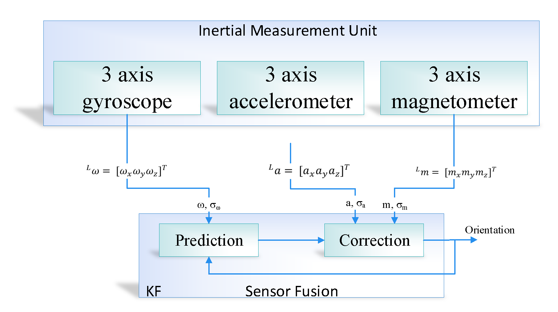
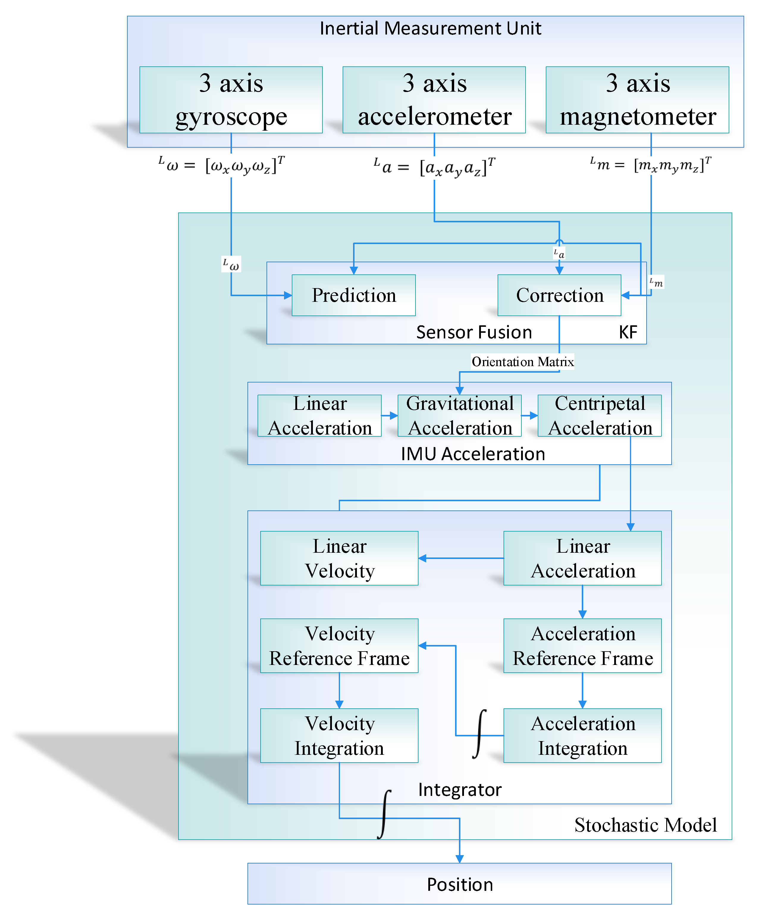
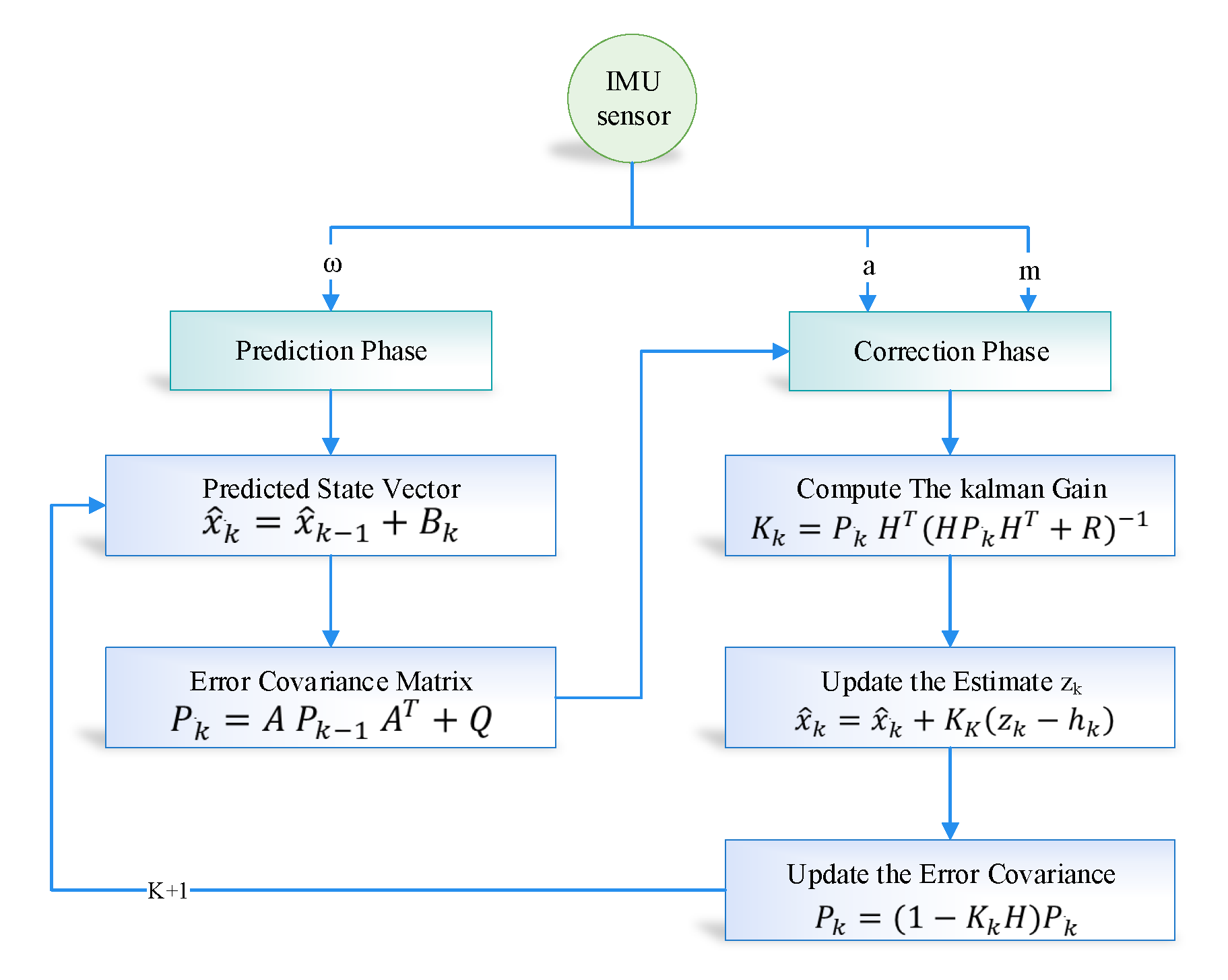
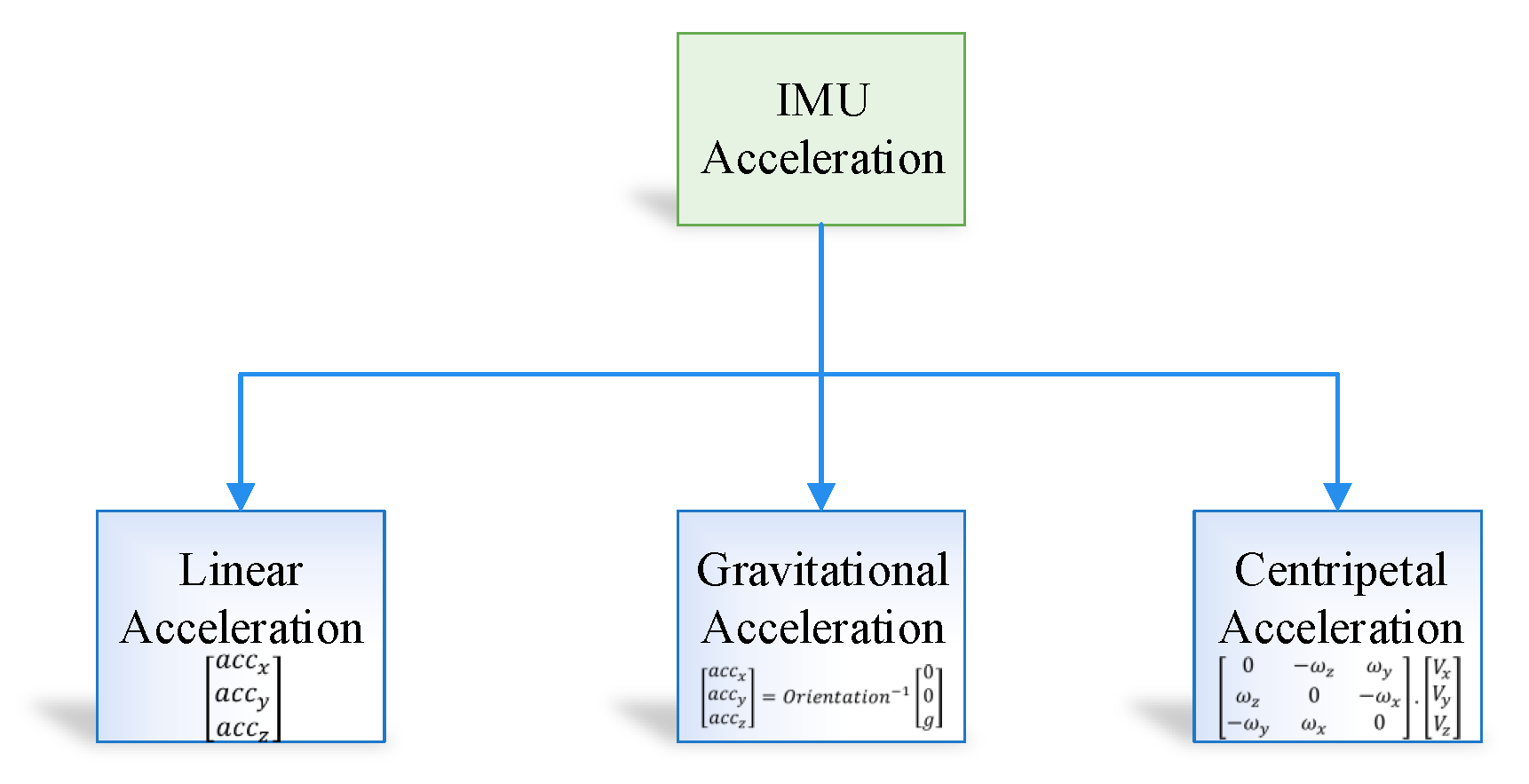
The proposed system is developed in order to evaluate the performance of the prediction algorithm, that is, the Kalman filter with the learning module. The experiment was performed on the real dataset taken in the engineering building of Jeju national university. At the start, the data were loaded into the application through NGIMU API. The data has ten inputs, that is, 3-axis accelerometer, 3-axis gyroscope, 3-axis magnetometer and time at which the data is taken. Afterwards, we calculated the orientation using sensor fusion based on the Kalman filter. The orientation matrix was further processed by removing the gravitational and centripetal forces and finally applied double integration to compute the position of an object in an indoor environment. Furthermore, the RMSE value of IMU sensor reading was computed by comparing its values with the actual IMU data such as the accelerometer and gyroscope sensor values. The RMSE for the IMU sensor reading was recorded as 5.25, which is considered very high.
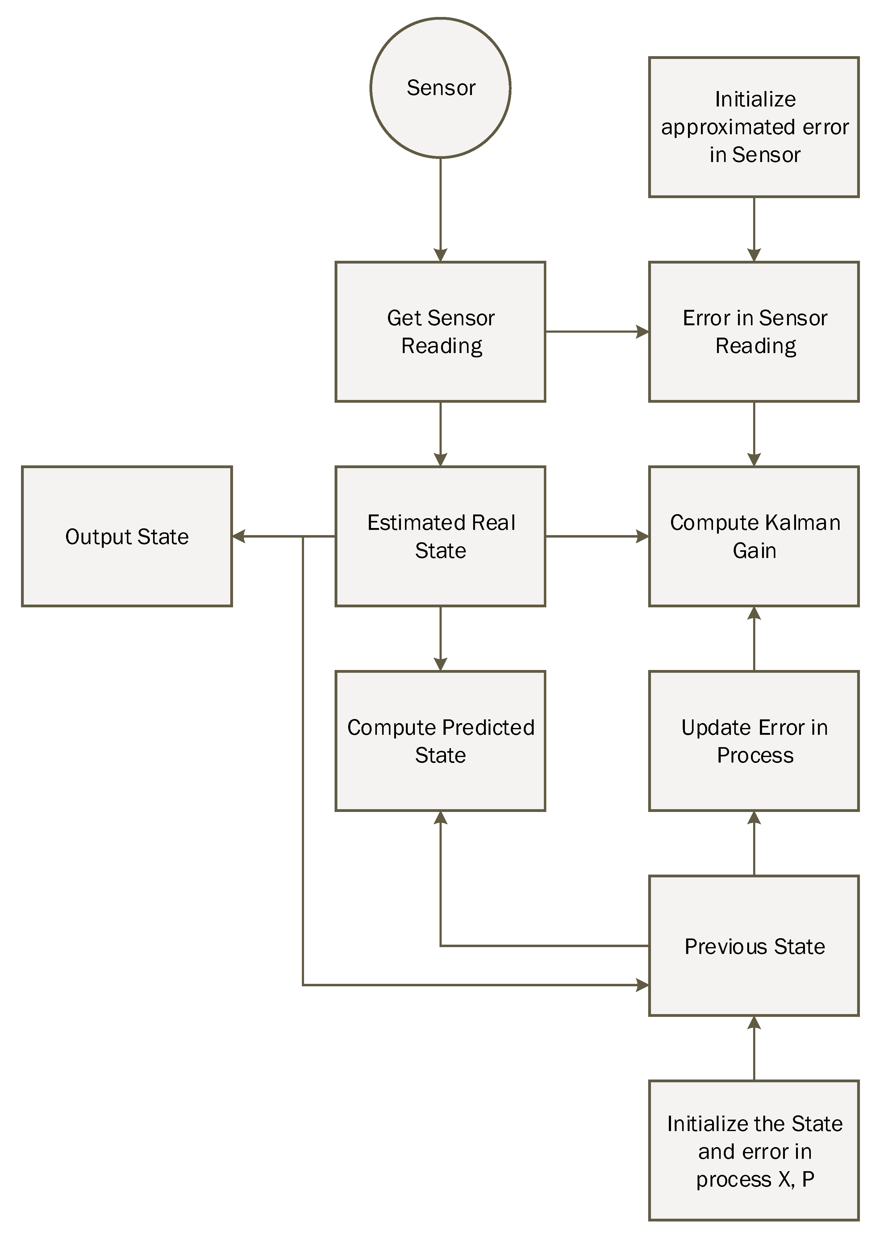
Moreover, we used a Kalman filter algorithm to forecast the actual sensor reading (i.e., accelerometer and gyroscope) form the noisy sensor reading. The develop interface provides manual training of the internal parameter of the Kalman filter, that is, the estimated error in measurement (R). Multiple experiments were carried out with different values of R in order to evaluate the performance of the proposed system. The RMSE of the predicted accelerometer and gyroscope was at . The predicted RMSE was better than the RMSE of sensor readings, that is, a 55% reduction of error.
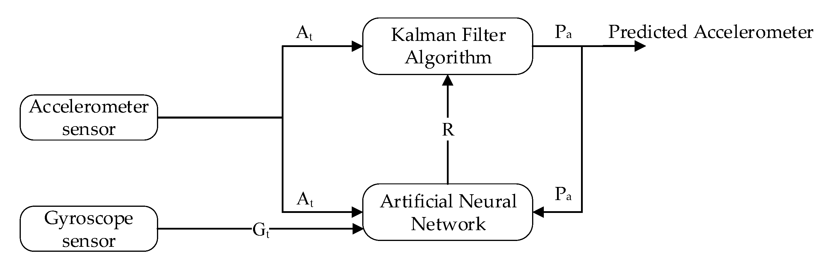
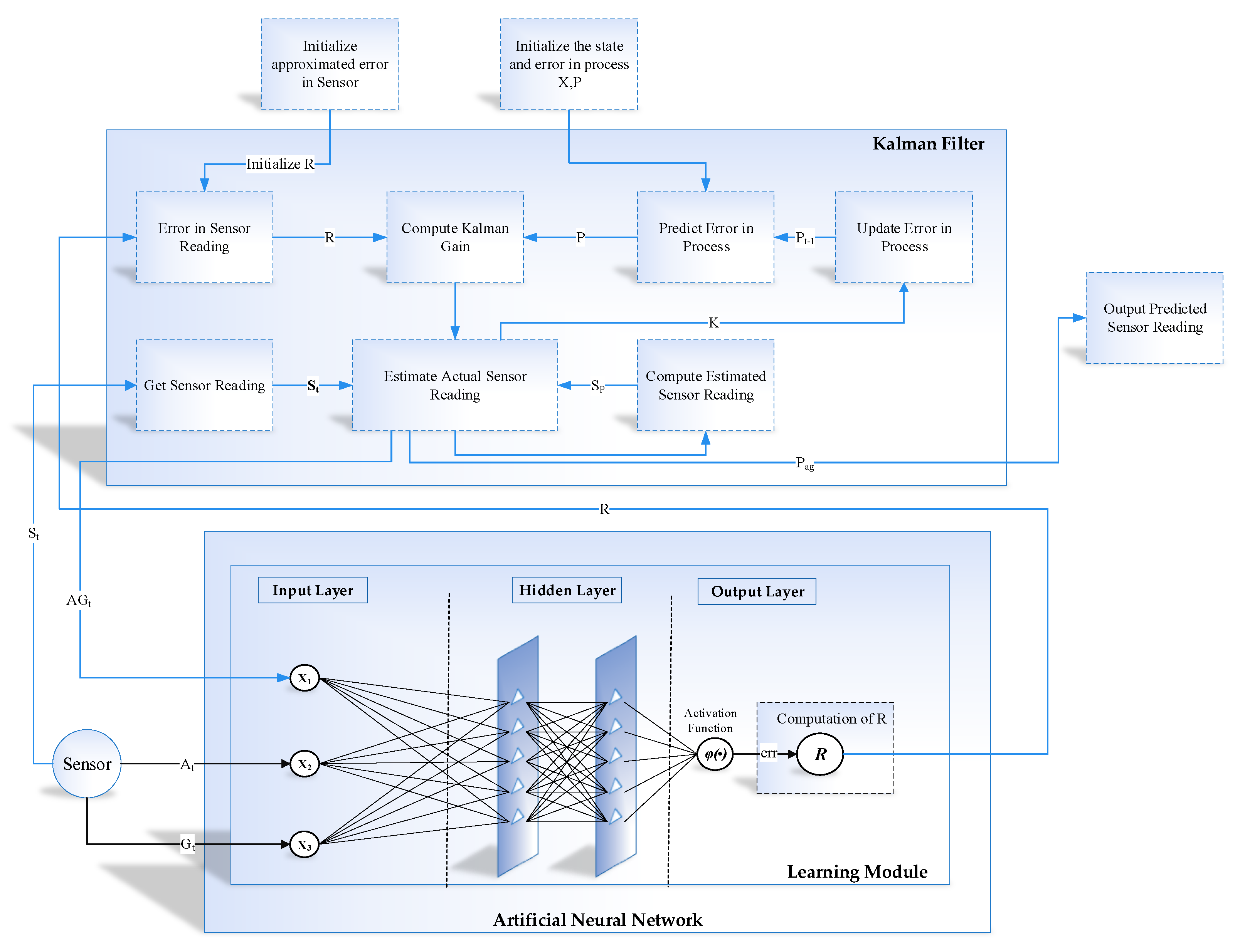
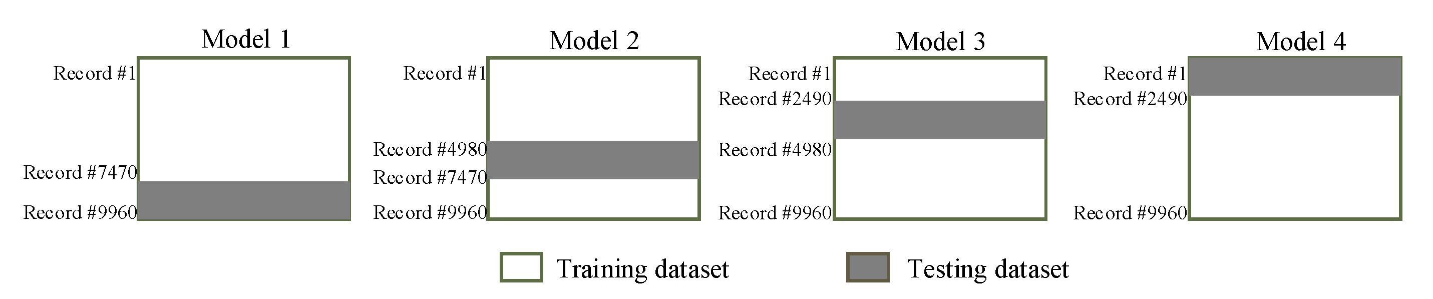
In the learning to prediction module, we had to use the ANN algorithm, which is used to enhance the accuracy of the prediction algorithm. The ANN algorithm was comprised of three neurons as an input layer and one neuron as a layer (i.e., accelerometer, gyroscope and Kalman filter predicted reading) and predicting the error in the sensor reading, respectively. Furthermore, we used n-fold cross-validation in order to avoid bias in the training process. For this purpose, we split the dataset into four equal subsets (i.e., 2490 samples in each subset) as shown in
Figure 11. According to 4-fold validation, 75% of the dataset was used for training, and other 25% was used for testing the ANN algorithm. Furthermore, in the proposed system, we used 100 epochs which were used for training the ANN algorithm. In the ANN-based learning module, the data normalization was done using Equation (
23).
where
is the normalized value for the
position of the input and output parameters, that is, accelerometer, gyroscope and predicted sensor data. The maximum and minimum value for each parameter in the dataset is denoted by
and
. Traditionally, in ANN training is done using normalized data, therefore in order to compute the predicted error we de-normalized the output data of the neural network using Equation (
24).
Furthermore, the proposed model accuracy was evaluated using three different matrices such as mean absolute deviation (MAD), root mean squared error (RMSE), and mean square error (MSE) as shown in Equations (
25)–(
27).
where total observation is denoted as
n, the target value is represented as
T, and
indicates the estimated value.
4.3. Results and Discussion
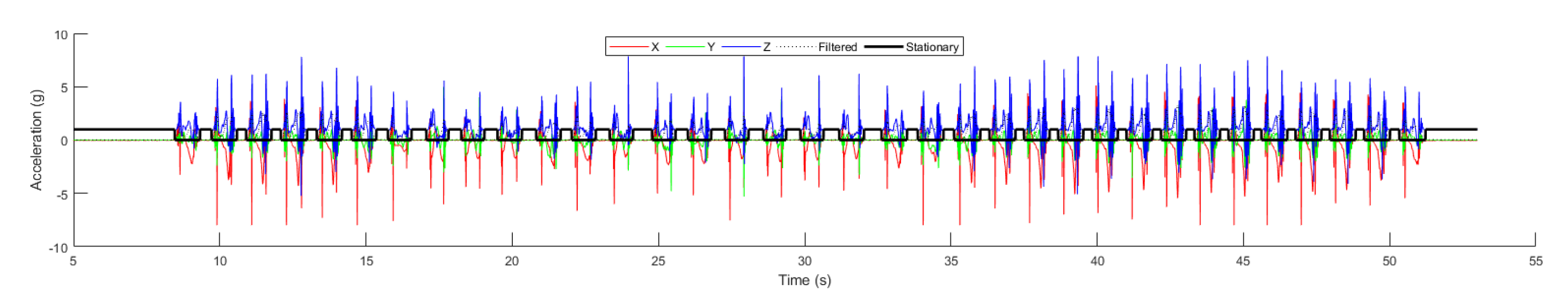
The open-source NGIMU was used to acquired data in order to calculate the object position in an indoor environment. Moreover, for analyzing the proposed system performance, we compared the result predicted by the conventional Kalman filter algorithm with the learning to prediction model. In
Figure 12, the raw accelerometer data is shown, which was acquired from the next-generation inertial measurement unit along with the time at which the data were taken. The 3-axis representation of the accelerometer data is denoted by x, y, and z. The dotted line represents the filtered data using a Butterworth filter based on the defined cut-off frequency, and the solid black line shows the stationary data, which is the magnitude of 3-axis acceleration. The stationary data represent the state of the object if the magnitude is less than
; the object state is stationary; otherwise, the object is moving.
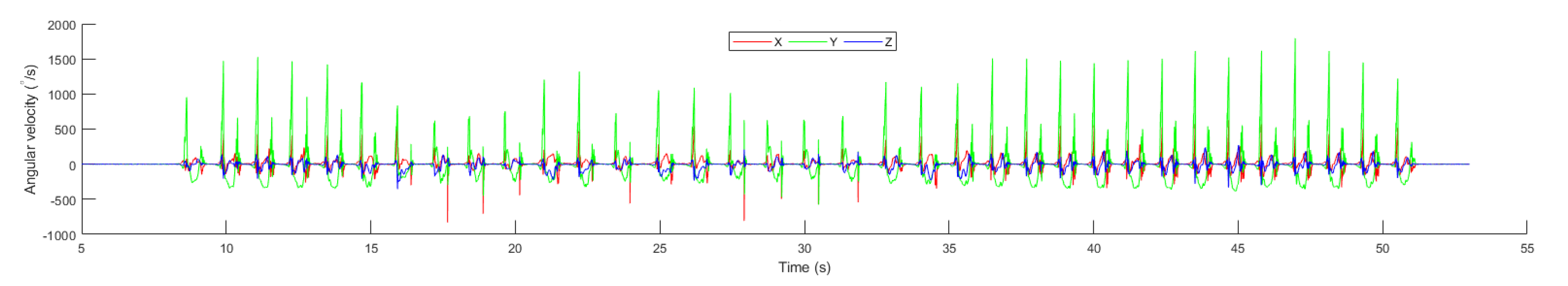
Figure 13 shows the value of the gyroscope, through which we calculated the value of the angular velocity of the moving object. The 3-axis gyroscope is represented by x,y, and z. The first integration of the angular velocity with respect to time leads to Euler angle, which is required to define the orientation of the object. The Euler angle is usually used to calculate the Roll, Pitch, and Yaw. The angular velocity is the rate of change in prescription of the object moving over time. The formula of angular velocity is mentioned in Equation (
28).
where
and
denotes the final angle and the initial angle of the object. The change of angle is denoted by
, and finally t represents the time.
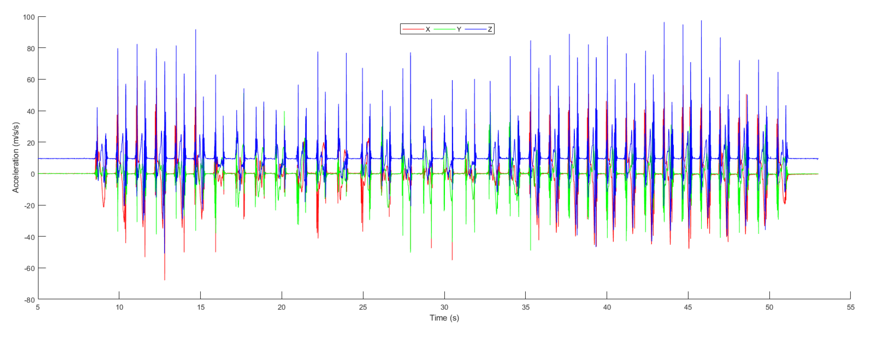
Figure 14 illustrated the acceleration
of the object in an indoor environment. The acceleration
of the object is measured as the rate of velocity over time and is calculated using the formula mentioned in Equation (
29)
where
denotes the change in velocity, a represent the acceleration in
and time is denoted by t.
The velocity of the object was measured as to how fast the object is moving in an indoor environment.
Figure 15 illustrated the 3-axis velocity of the object, which is calculated using the formula mentioned in Equation (
30).
where
represents the change in position of the object within an indoor environment,
v denotes velocity and
t represents the time at which the object changes its position.
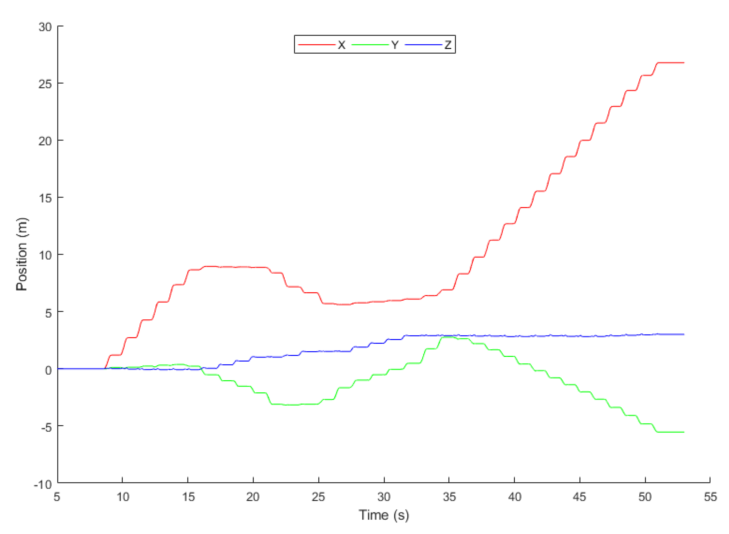
In
Figure 16, the 3-axis position of the object is represented using a 2-dimensional graph where x, y, and z represent the axis.
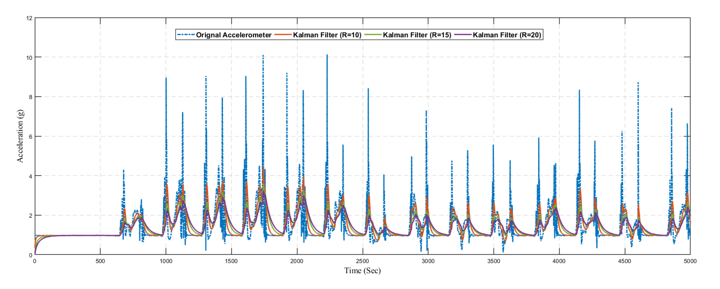
In
Figure 17, we present the predicted result of the accelerometer sensor using the traditional Kalman filter without the learning model. We compared the original sensing data with different values of
R. The optimal value of
R is based on the dataset, and it is not fixed. Hence it is difficult to find the optimal value of
R manually, so we considered different values of
R. Also from the graph, it can be seen that the Kalman filter prediction accuracy changed with changing the values of
RSimilarly,
Figure 18 shows the result of predicted angular velocity using a conventional Kalman filter without the learning model. The graph represents the variation in prediction results by varying the value of
R in the Kalman filter configuration. The gyroscope sensor reading is predicted using three different configurations as summarized in
Table 5.
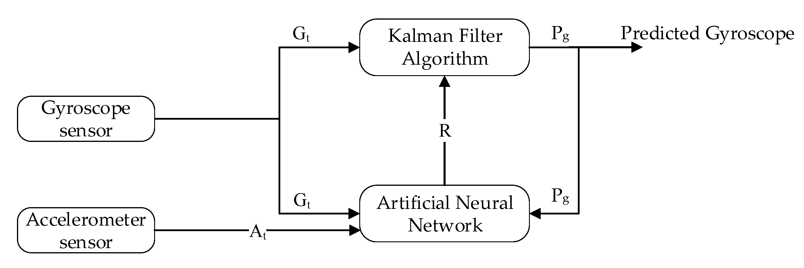
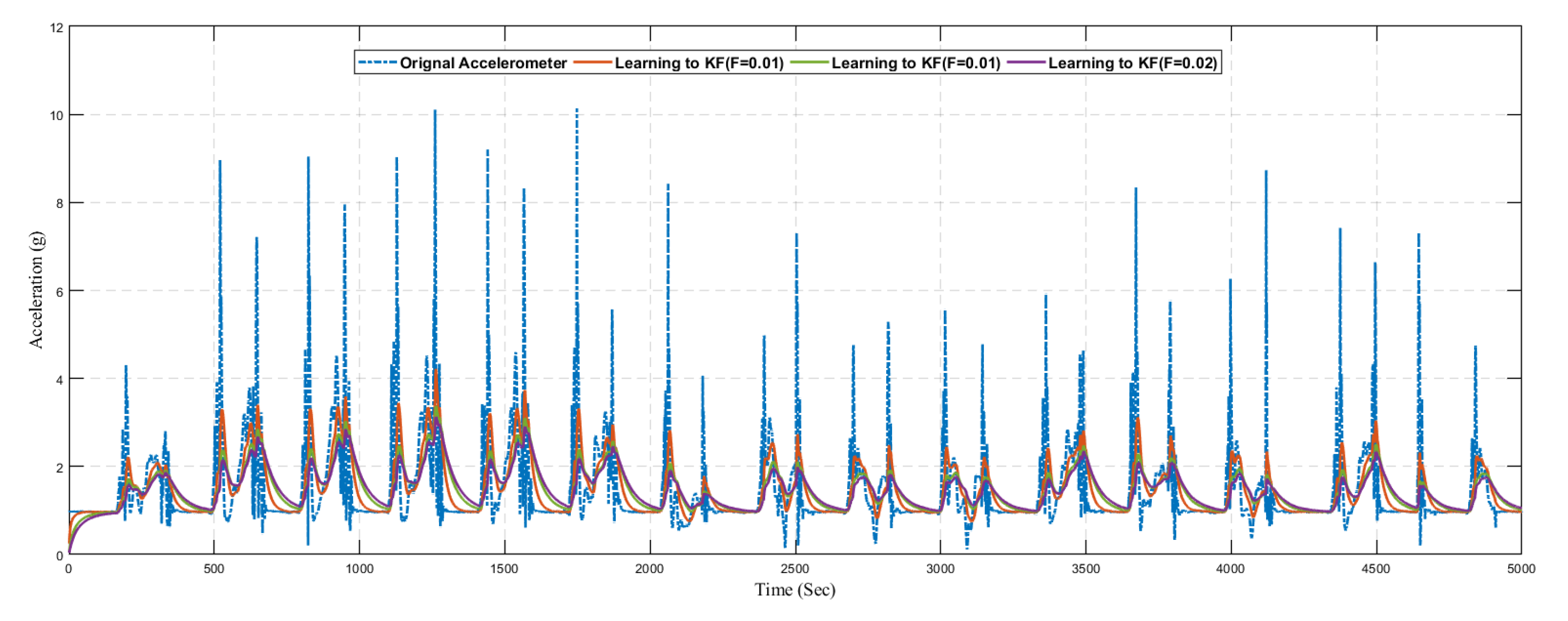
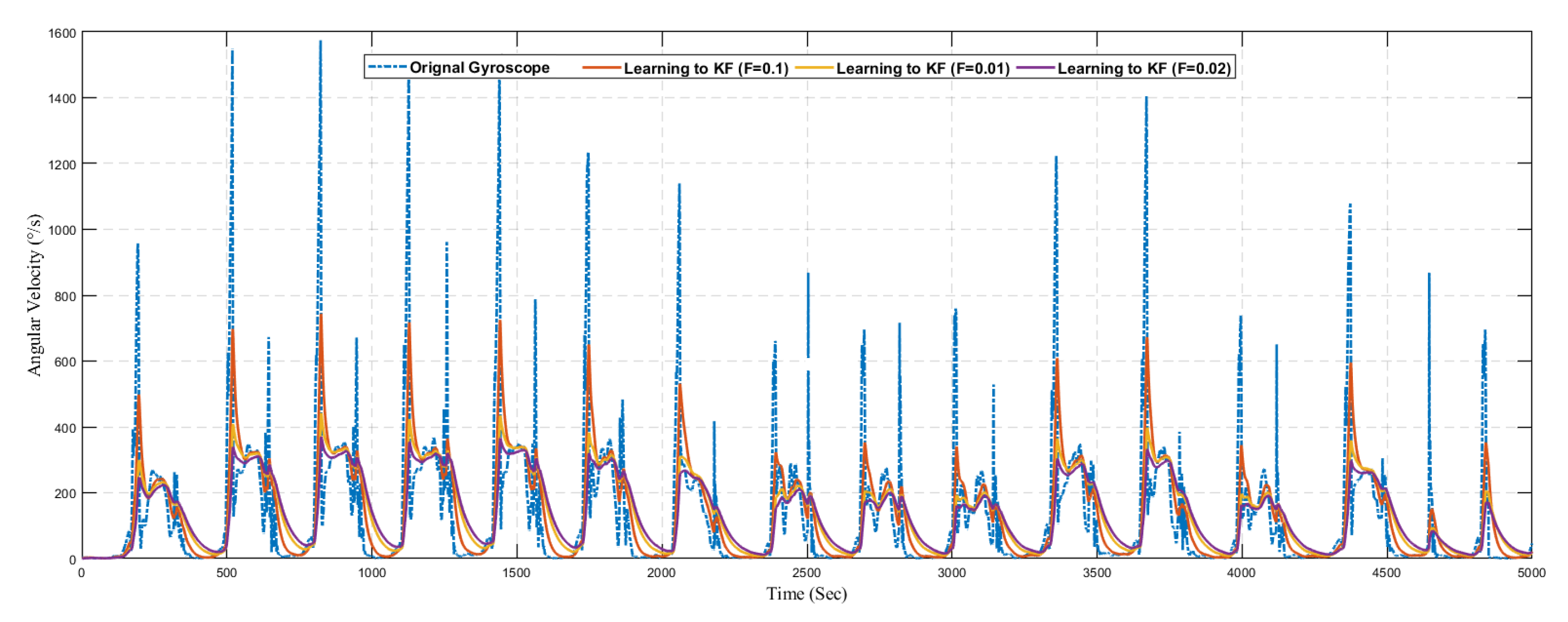
Next, we present the results of the proposed learning to prediction for both accelerometer and gyroscope sensors readings, as illustrated in
Figure 19 and
Figure 20. We used the ANN trained model in order to improve the performance by tuning its
R parameter. The predicted error rate update the R for the Kalman filter algorithm based on
R; we choose the suitable value for
F, also called the error factor using Equation (
31).
where proportionality constant also called as error factor denoted as
F.
The graph shows the position data for 60 s in which the first 10 s represents the stationary state. If we investigated the position plot, then we came to know that the proposed system significantly reduced the drift and error from the sensing data.
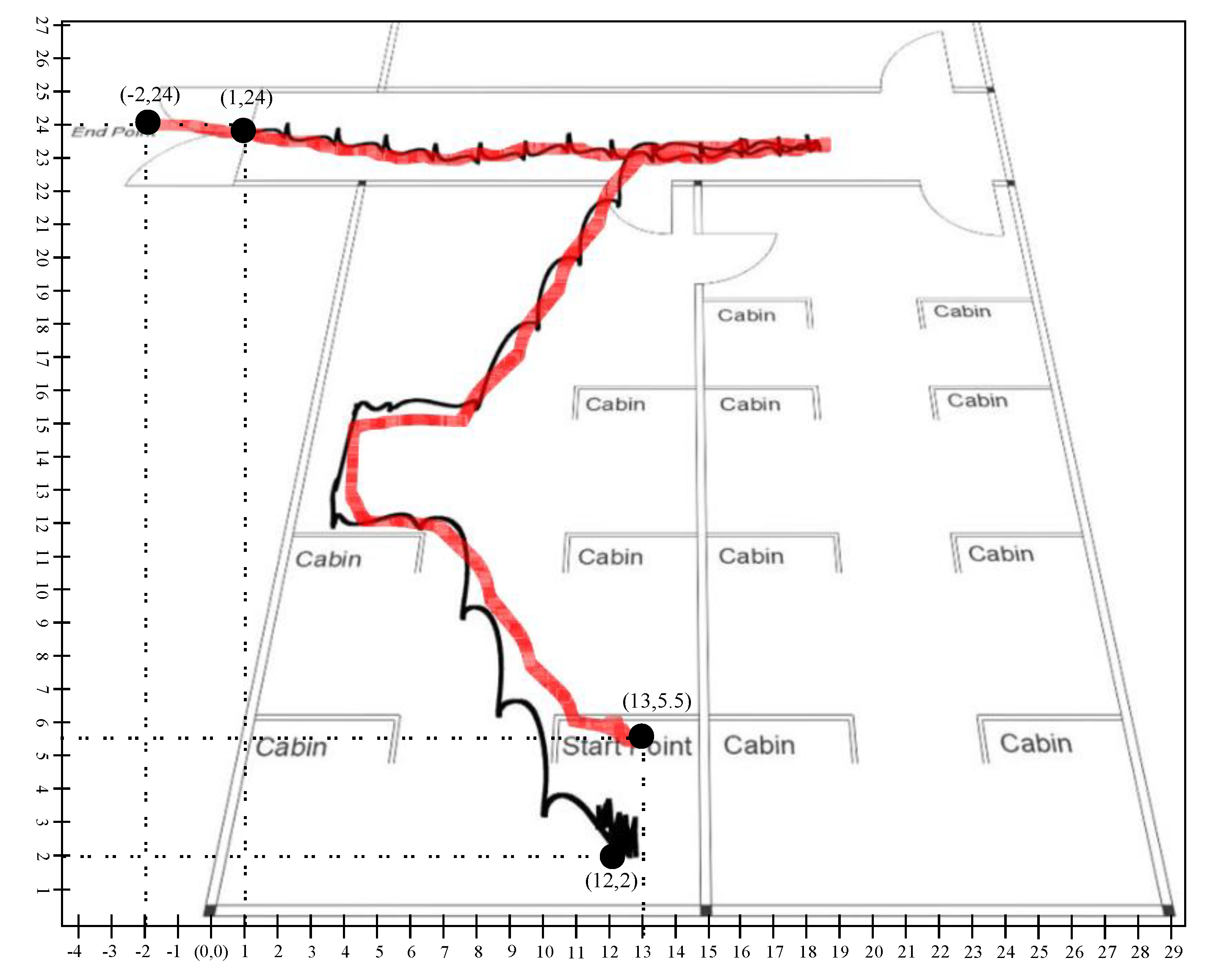
Figure 21 and
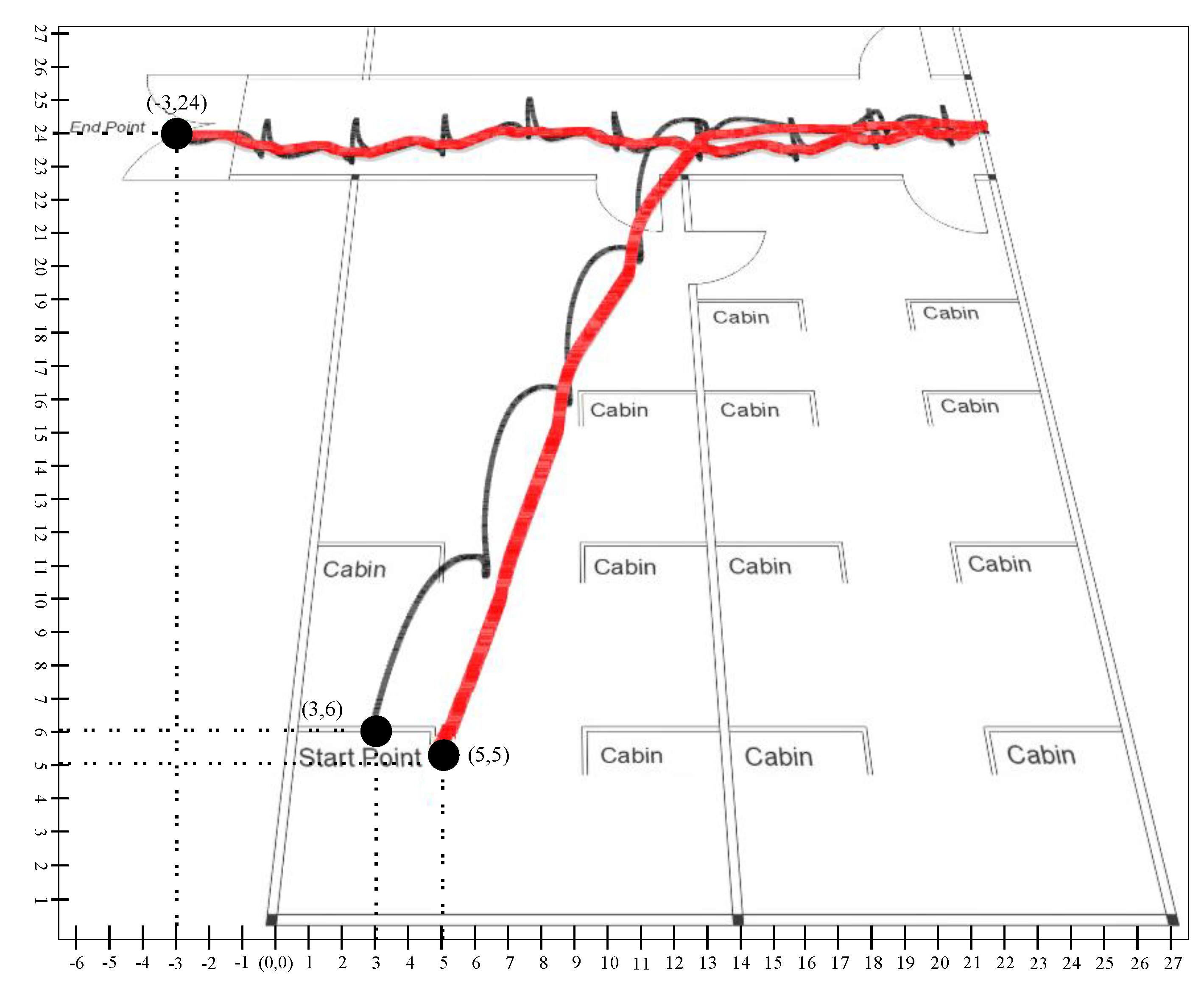
Figure 22 illustrated the trajectory of a person walking in room no D242 toward the main corridor. In both scenarios, the person starts walking from the starting point where the first 10 s remained stationary so that the algorithm could converge on a stable state and stop walking at the endpoint in the main corridor. The black line shows the trajectory of the person calculated using a stochastic model, that is, position estimation using sensor fusion, whereas the red line is the predicted trajectory using the learning to prediction model. As we see in the results that the amount of drift in the sensor reading is greatly reduced after tuning prediction algorithms using artificial neural networks. In scenario 1, illustrated in
Figure 21, the starting point is
and the endpoint is
computed using traditional Kalman filter with respect to defined reference point
. Similarly, in the case of learning to Kalman filter model, the accuracy of the indoor system is improved in which the starting point and the ending point are
and
receptively. All the computed coordinates are mapped according to the defined reference point
.
Similarly in scenario 2, presented in
Figure 22, we compute the result of the conventional Kalman filter with
as a starting point, and the ending point is mapped as
as x-coordinate and 24 as y-coordinate with
reference point. For the learning to prediction model, the accuracy is improved with respect to reference point
, where the start point is mapped as
and the endpoint is
.
Table 6 presents the RMSE in position with the prediction model and the learning to prediction model. The results indicate that the error in position estimation is improved by 19% in the case of the learning to prediction model. Furthermore, the proposed model precise the sensor reading based on bias error correction, which results in improving the system accuracy.
As it was challenging to differentiate the result presented in
Figure 19,
Figure 20,
Figure 21 and
Figure 22. Thus, there is a need for several statistical methods to evaluate the above-presented results in a single quantifiable comparative analysis as mentioned in Equations (
25)–(
27). We have conducted multiple results for evaluating the performance of a traditional Kalman filter with different
R values. Likewise, in the case of the learning to prediction module, the performance is assessed with the selected value of error factor (f). Experimental results show that Kalman filter with learning to prediction module with
performed well as compared to other statistical measures. The best outcome for the Kalman filter with no learning module where
, as a result of
prediction accuracy in terms of RMSE. Similarly, the best case for the learning to prediction module is recorded with
, with a result of
prediction accuracy in terms of RMSE. Significant enhancement in the prediction accuracy of the learning to prediction module as compared to the Kalman filter with the learning module is 0.041% for the best case and 0.11% for the worst case in terms of RMSE. The statistical summary of Kalman filter for both learning and without learning module is summarized in
Table 5.


