Characterization of FIREFLY, an Imaging Spectrometer Designed for Remote Sensing of Solar Induced Fluorescence


Abstract
:1. Introduction
2. Materials and Methods
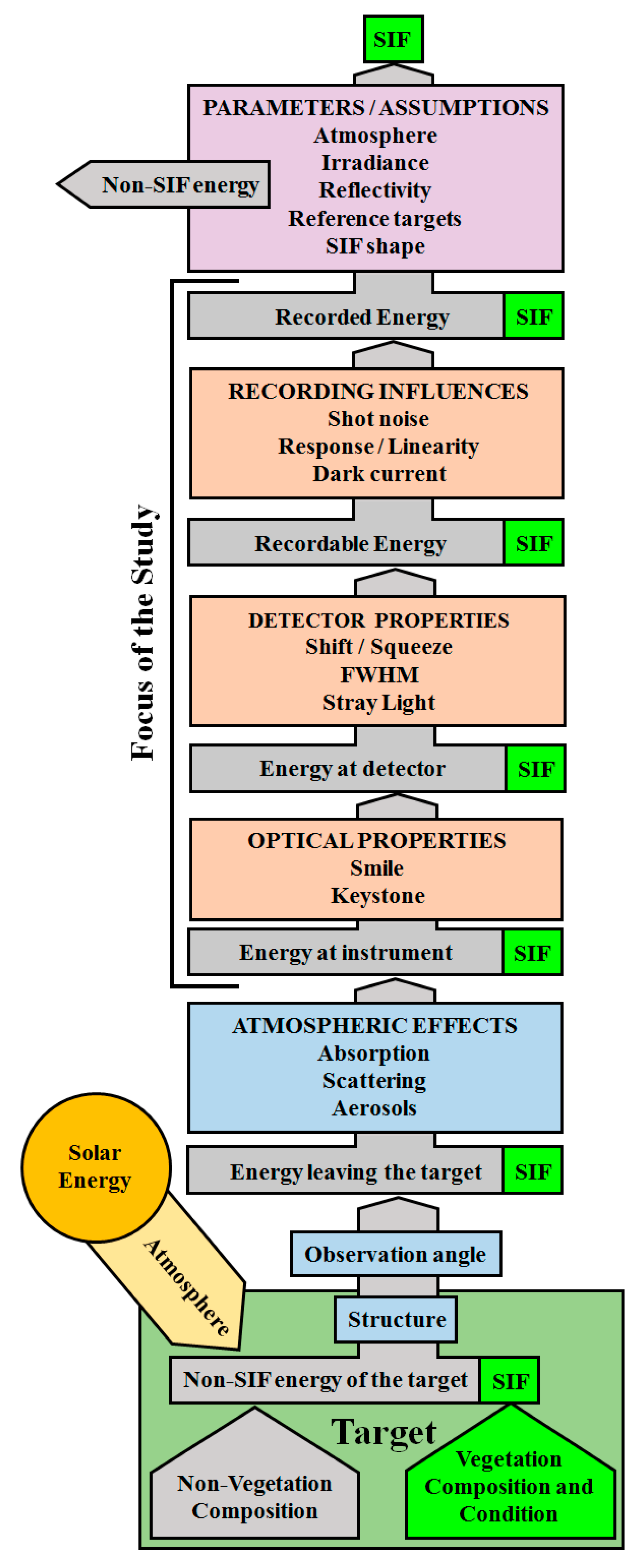
2.1. Representing SIF Retrieval Methods
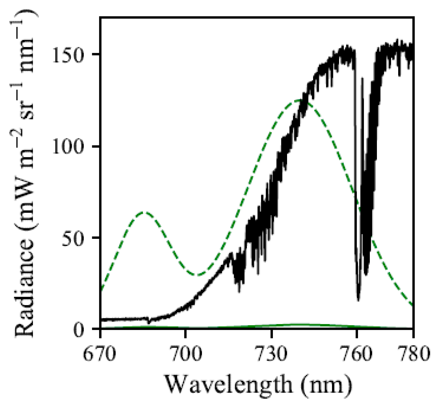
2.2. Representing SIF Signals
2.3. Representing FIREFLY Spectra
2.3.1. Deriving Baselines for Indirect SIF Retrievals
2.3.2. Forward Modelling with Simulated Spectra
2.4. Characterizing FIREFLY with GLAMR
2.5. Characterizing FIREFLY with Integrating Sphere
2.6. Characterizing FIREFLY with Controlled Acquisitions
2.7. Characterizing FIREFLY with In-Flight Acquisitions
3. Results
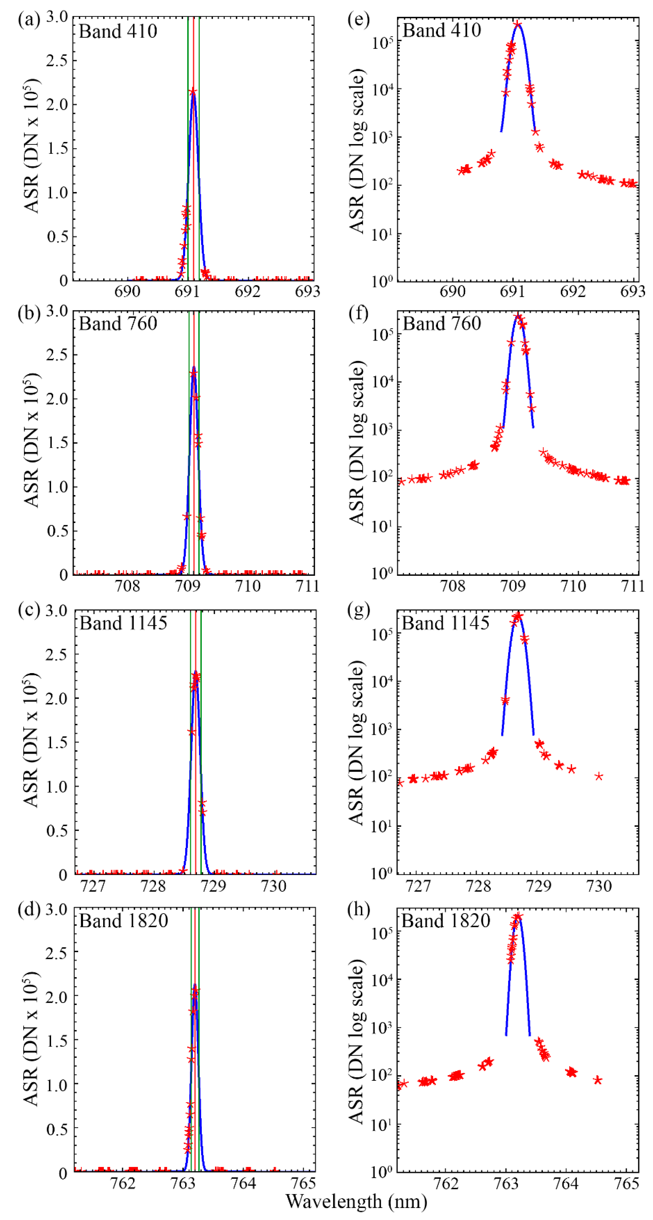
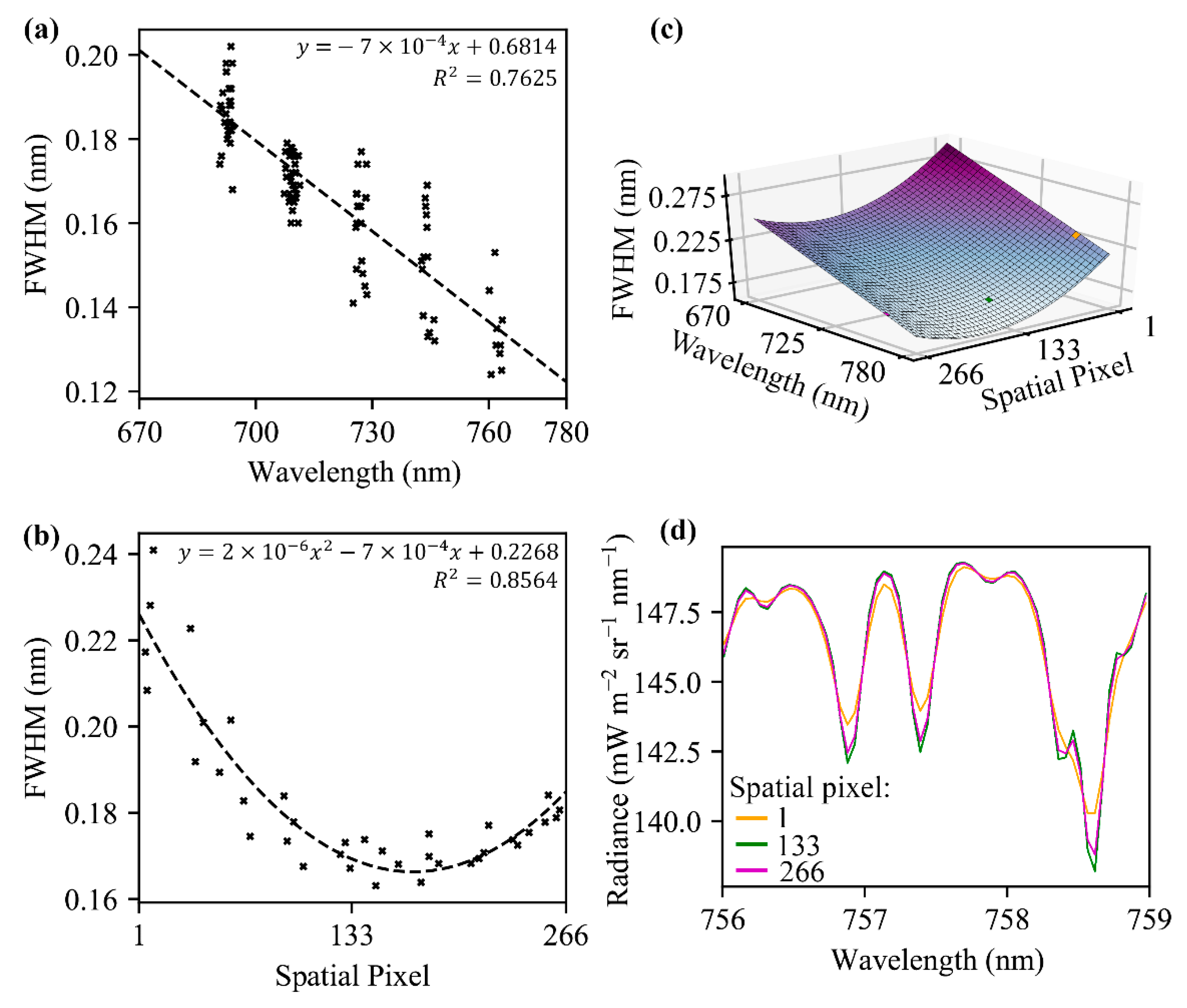
3.1. Spectral Channel FWHM
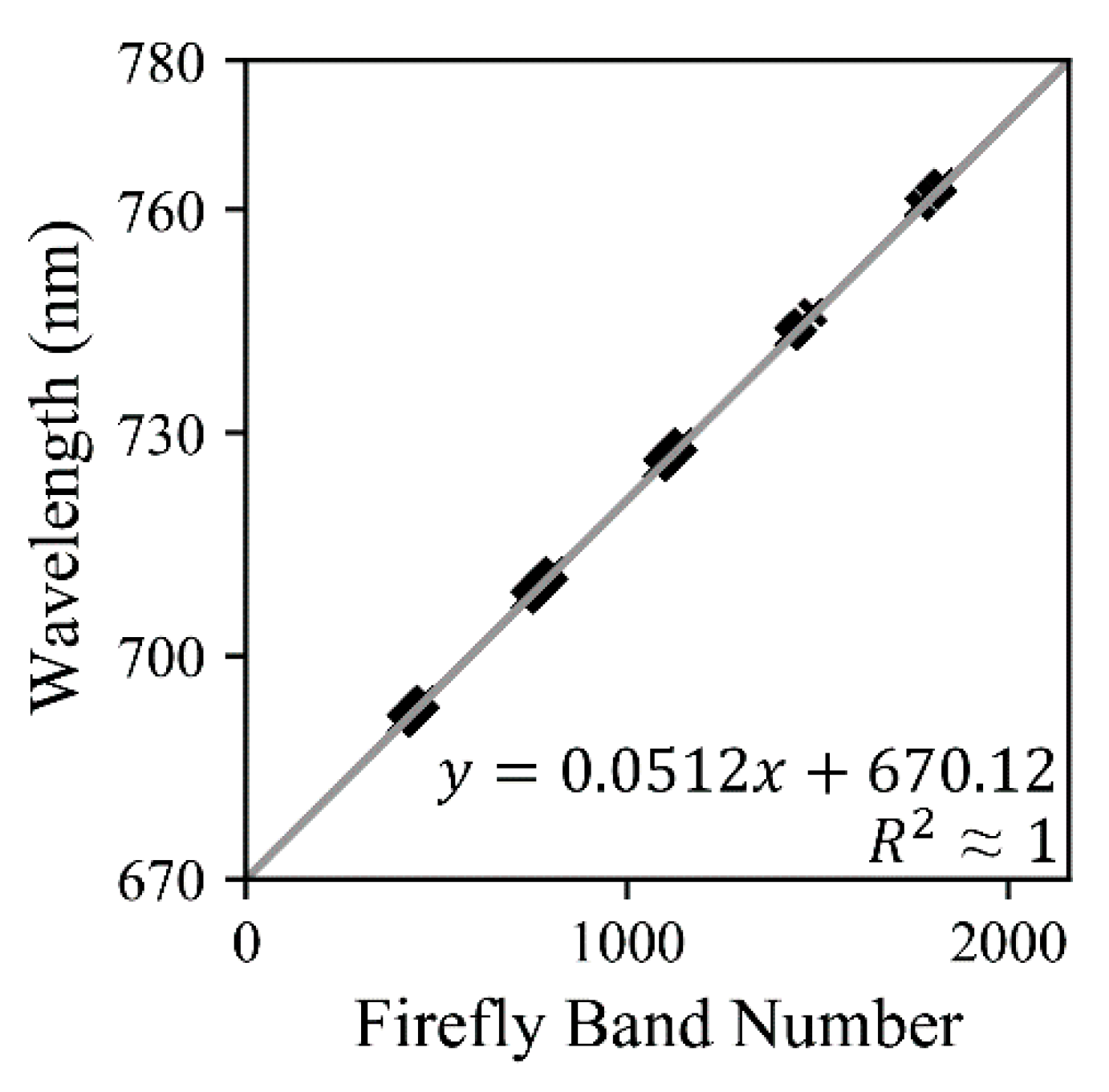
3.2. Band Centers
3.3. Detector Response and Linearity
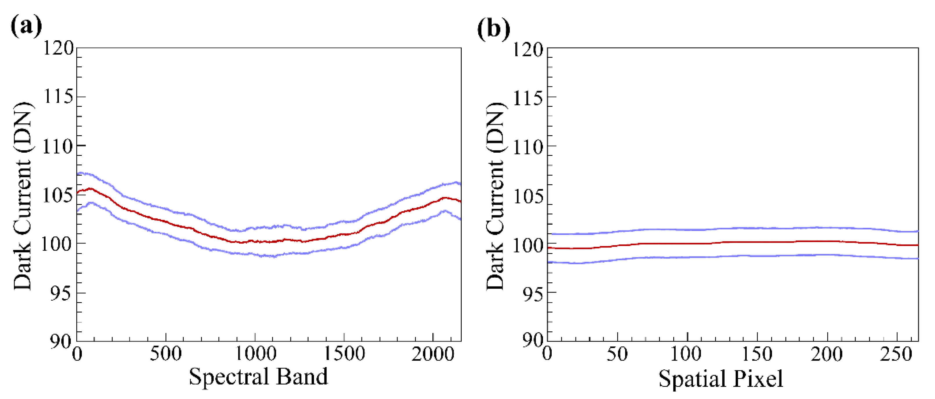
3.4. Dark Current
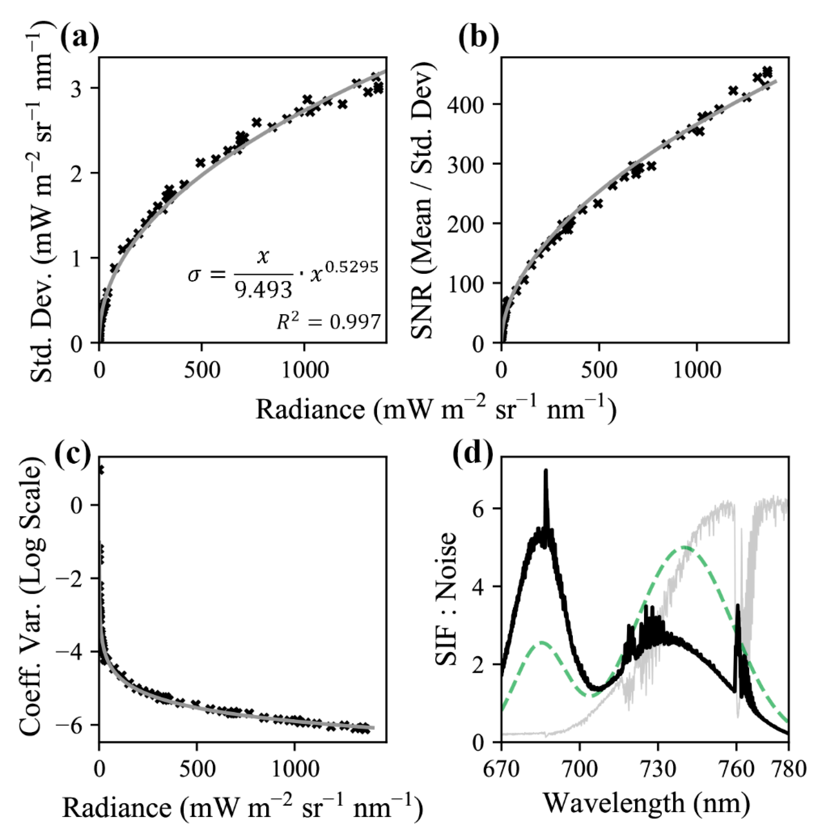
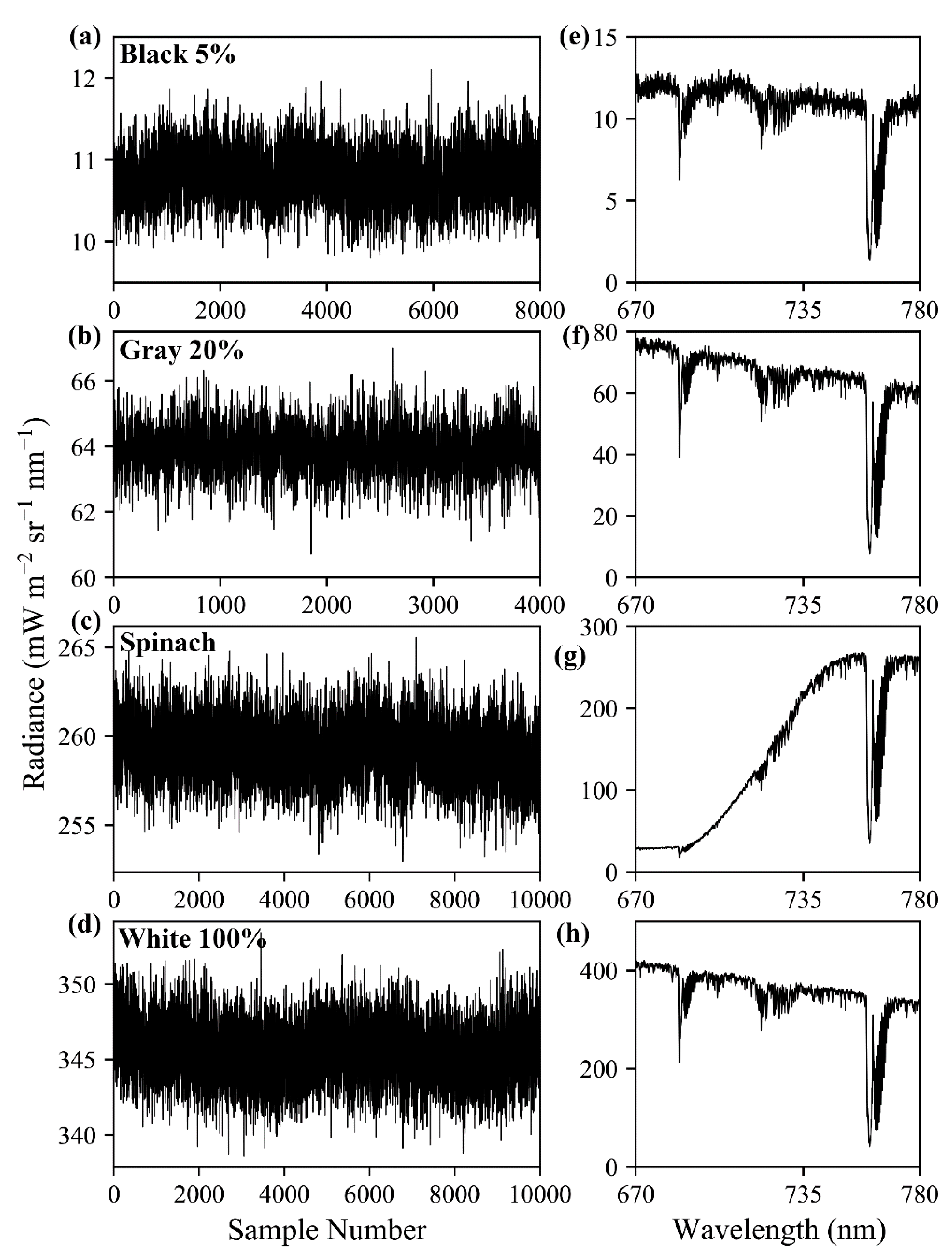
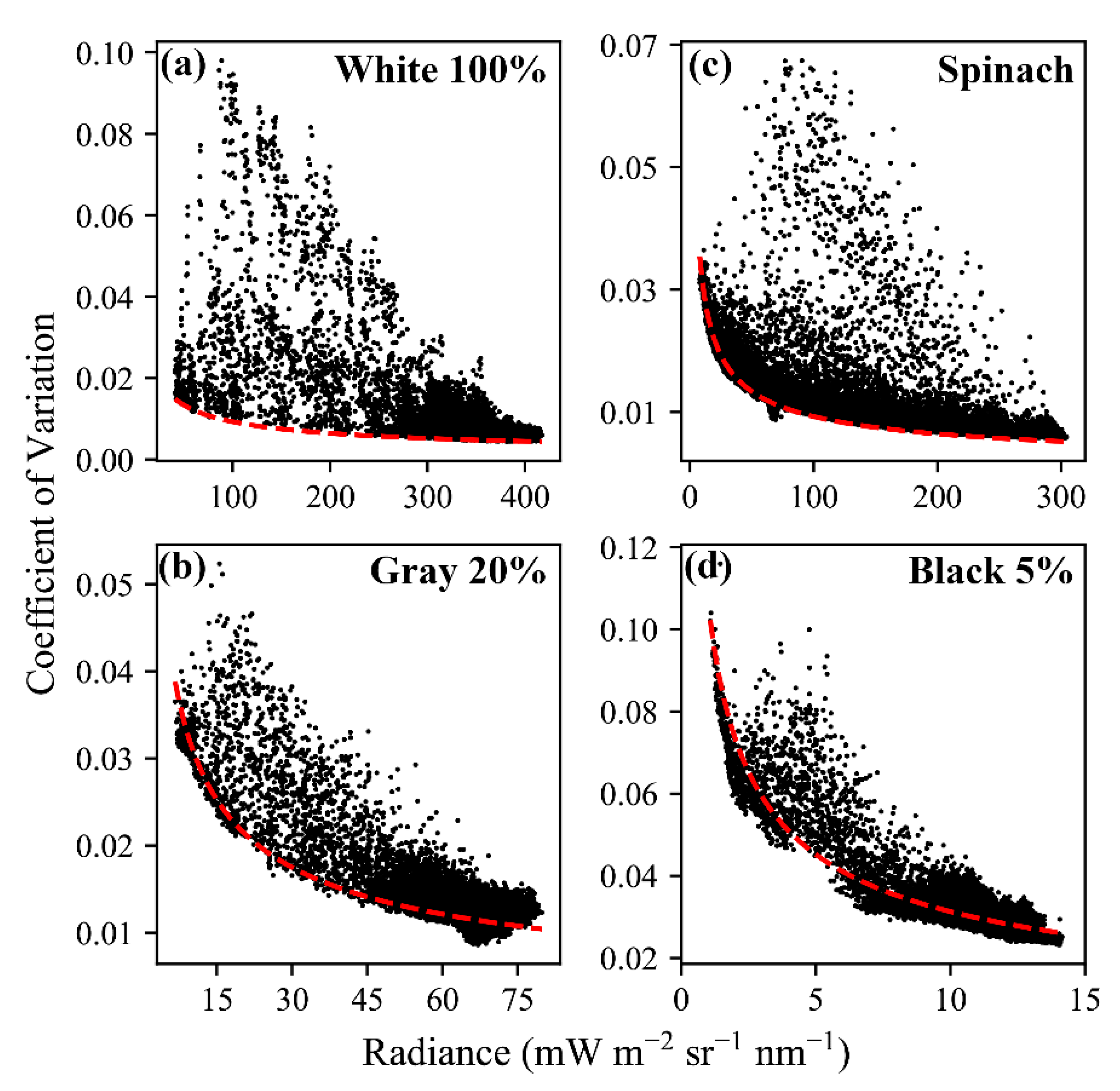
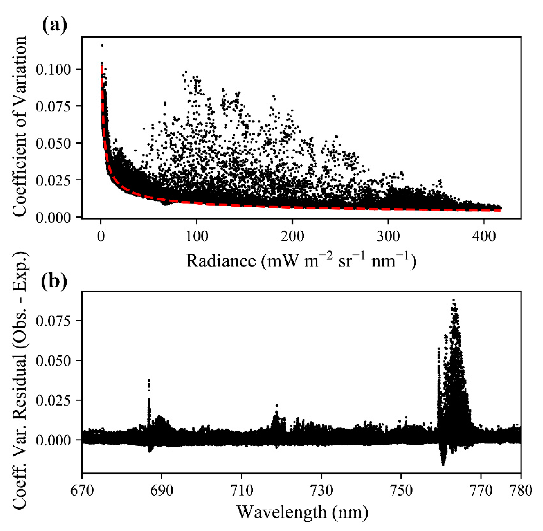
3.5. Shot Noise
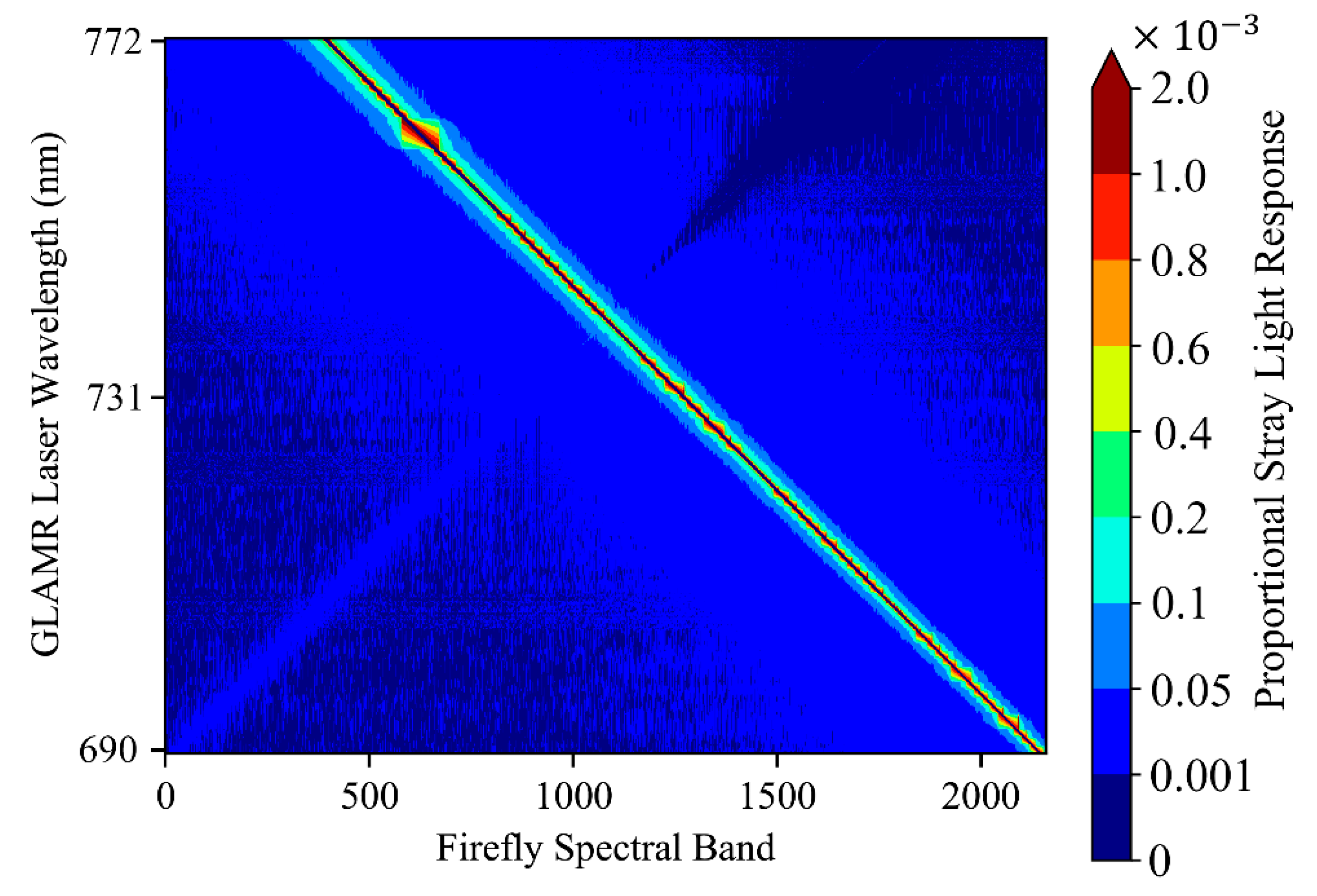
3.6. Stray Light
3.7. Forward Modelling
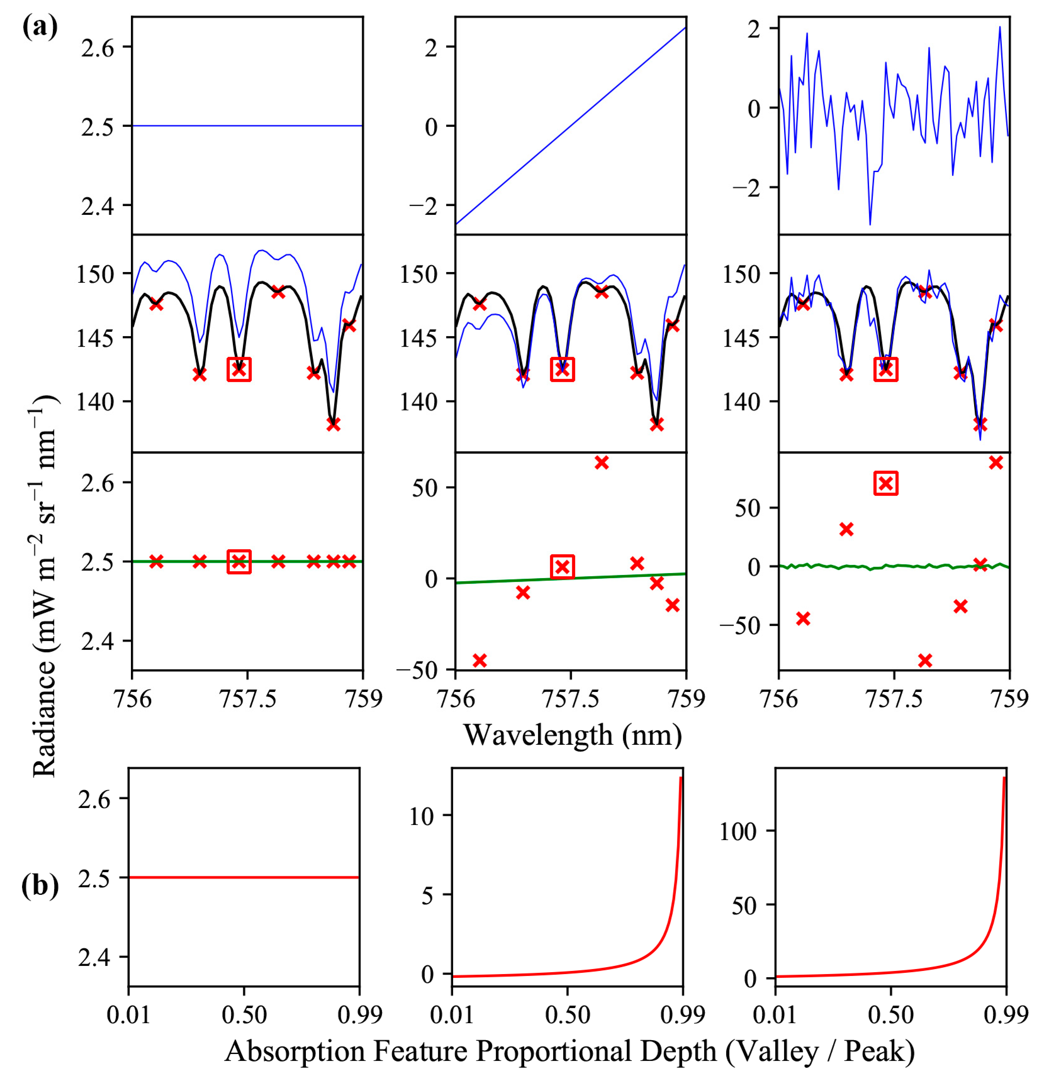
- Uniform influences on spectra intended for SIF retrieval will result in one-to-one error in both direct and indirect SIF retrievals (Figure 3).
- Non-uniform sloped influences produce one-to-one error in direct retrievals (Figure 3).
- All non-uniform influences produce amplified errors in indirect SIF retrievals (the magnitude of the error is higher than the sum of the influences on the relevant bands) (Figure 3).
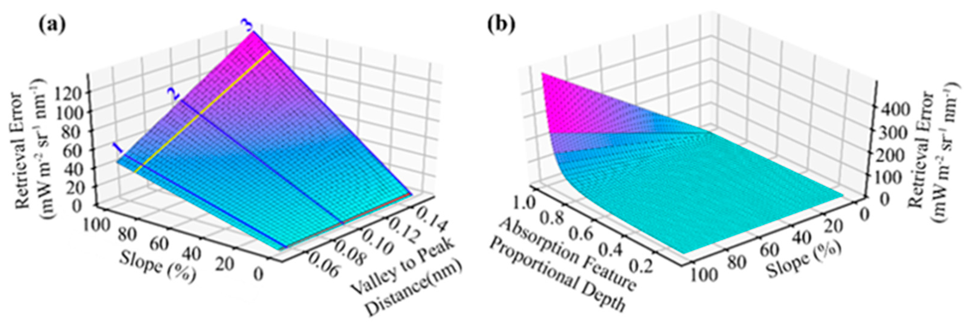
- Sloped influences produce positive errors in indirect SIF retrievals if the direction of the slope increases the valley radiance relative to the peak radiance, and negative errors if the peak is increased relative to the valley.
- Sloped influences produce higher magnitude errors in indirect SIF retrievals when there is a steeper slope; when the spectral distance between the valley band and the peak band is greater; or when the absorption feature is shallower (the proportional depth is higher) (Figure 14).
- Random influences produce one-to-one error in each band used for direct retrievals (Figure 3).
- Random influences that are expected to be normally distributed (such as shot noise) produce bimodal error distributions in indirect SIF retrievals (Figure 15).
4. Discussion
4.1. SIF Retrievals with FIREFLY
4.1.1. Indirect Retrievals from Solar and Oxygen Absorption Features
4.1.2. Direct Retrievals
4.2. Interpretation of SIF Retrievals
5. Conclusions
Supplementary Materials
Author Contributions
Funding
Acknowledgments
Conflicts of Interest
Appendix A
Appendix A.1. Indirect Retrievals
Appendix A.2. SIF Signal Simulation
Appendix A.3. Modelling Tools and Code
- Absorption_Feature_Peaks.py contains a function “get_abs_feat” to return a set of absorption features and their relative depths. Additionally, contains a function “get_abs_feats_set” to return a set of absorption features filtered by spectral region, spatial pixel, or maximum band offset between valleys and peaks.
- Data_Loader.py contains a function “load_instrument” that creates an instance of the instrument class, and then uses the method to import a saved JSON file for an instrument into the instance. Additionally, contains a function “load_data” that loads specific JSON data files based on which other function calls it. There is a function “load_*” for each major dataset that imports the JSON file for the dataset via the “load_data” function.
- ENVI_File_Import.py contains a function “envi_read” that imports an ASCII file exported from ENVI as a Python dictionary.
- Instrument_Builder.py contains the class “Instrument” to represent an instrument for SIF retrieval in analyses. The class contains methods “import_instrument” to import the instrument from a saved JSON; “export_instrument” to export the instrument to a JSON, which is called on initialization of an instance of the class; “normcdf” to return a proportion from a normal cumulative distribution function for a given location of a normal distribution based on a given mean and standard deviation; “convolve” to sample high resolution reference spectra according to instrument specifications; “simulate_spectra” to simulate a set of spectra covering all the spatial pixels of the instrument; “abs_feat” to derive a set of absorption features from simulated spectra; “get_band_wl” to return the wavelength of a band in nanometers based on an input band number; and “get_band_num” to return a band number based on an input band wavelength.
- Keys_As_Sorted_Floats.py contains the function “get_key_floats” that returns a list of band wavelengths as floats and a list of bands as strings based on an input set of dictionary keys. Additionally, contains the function “get_key_ints” that returns a list of band wavelengths as integers and a list of bands as strings based on an input set of dictionary keys.
- SIF_Estimate.py contains the function “integrate_SIF” to return a range of wavelengths for an evaluation of SIF, an estimate of the absolute SIF in each of a list of input bands, and an estimate of the total SIF across all of the input bands. Additionally, contains the function “get_sos_residual” that takes an estimated SIF signal and an expected SIF signal and returns the sum of the squared residuals between the two. Additionally, contains the function “estimate_sif” that returns the values for SIF at as set of wavelengths, and the residual based on the best fit of an input set of SIF estimates to the SIF simulation key parameters (see Appendix A.2) as independent variables, and the sum of the squared residuals as the response variable.
- SIF_Simulation.py contains the function “simulate_SIF” to provide a SIF signal derived according to Appendix A.2. Additionally, contains the function “get_sif” to provide a SIF estimate at a given wavelength based on a simulated SIF signal.
- Spectral_Regions.py contains a function for each spectral region “in_*” to test whether a given band is in the spectral region in question, returning a True or False. Additionally, contains a function “all_regions” that returns a dictionary with keys named for each spectral region, and values of True or False to indicate whether a given band is in the spectral region.
- Wavelength_Band_Conversion.py contains the functions “get_bands_from_wl” and “get_bands_from_nums” that both return lists of band numbers and band wavelengths as floats, based on input lists of wavelengths and band numbers, respectively.
- Absorption_Feature_Search.py executes a series of methods on an instance of the instrument class to establish a set of absorption features for each spatial pixel found in the simulated spectra. The saved JSON file for the instrument is then updated.
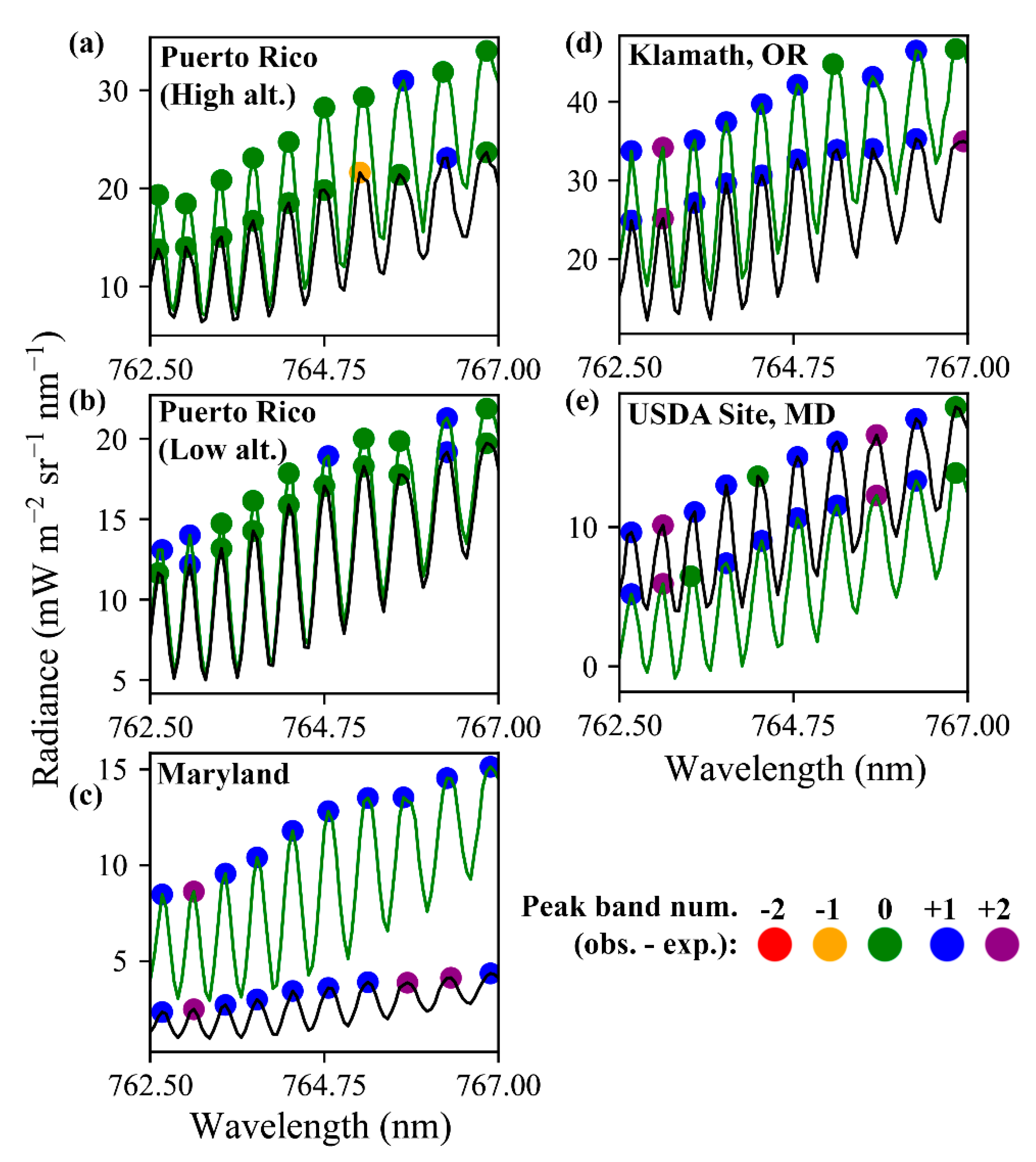
- Shift_Squeeze_Test.py prints a count of flags based on analysis of an input ASCII file exported from ASCII. The flags are based on analysis of the absorption features in the trailing region of the oxygen A feature, and return a yellow flag when the apex of a feature is found ± 1 band from the expected band, and a red flag when the apex is found ± 2 bands from the expected band.
- Simulate_Spectra.py executes a series of methods on an instance the instrument class to simulate spectra based on each spatial pixel. The saved JSON file for the instrument is then updated.

| Figure Number | Python Script |
|---|---|
| 1 | Figure_A.py |
| 3 | Figure_I.py |
| 5 | Figure_B.py |
| 6 | Figure_N.py |
| 7 | Figure_L.py |
| 9 | Figure_K.py |
| 10 | Figure_E.py |
| 11 | Figure_D.py |
| 12 | Figure_C.py |
| 13 | Figure_M.py |
| 14 | Figure_R.py |
| 15 | Figure_G.py |
| 16 | Figure_H.py |
| 17 | Figure_J.py |
| 20 | Figure_O.py |
| 21 | Figure_P.py |
| 22 | Figure_Q.py |
| 24 | Figure_F.py |
| Collect Name | ID | Location | Filename | Notes |
|---|---|---|---|---|
| Klamath OR | 1 | Oregon, USA | Klamath_OR | Outside Klamath Falls |
| Puerto Rico (High alt.) | 2 | Puerto Rico, USA | PR_BG_high_2k | High flight altitude |
| Puerto Rico (Low alt.) | 3 | PR_BG_low_2k | Low flight altitude | |
| El Verde, Puerto Rico, | 4 | PR_EV2_9k | El Yunque National Forest | |
| El Verde, Puerto Rico 2 | 5 | PR_EV2_11k | El Yunque National Forest | |
| Maryland | 6 | Maryland, USA | UAS_2017 | University of Maryland UAS Test Site |
| USDA Site, MD | 7 | USDA_OPE_0 | USDA Test Site | |
| USDA Site, MD 2 | 8 | USDA_OPE_1k | USDA Test Site |
References
- Cook, B.; Nelson, R.; Middleton, E.; Morton, D.; McCorkel, J.; Masek, J.; Ranson, K.; Ly, V.; Montesano, P. NASA Goddard’s LiDAR, hyperspectral and thermal (G-LiHT) airborne imager. Remote Sens. 2013, 5, 4045–4066. [Google Scholar] [CrossRef] [Green Version]
- Frankenberg, C.; Fisher, J.B.; Worden, J.; Badgley, G.; Saatchi, S.S.; Lee, J.E.; Toon, G.C.; Butz, A.; Jung, M.; Kuze, A.; et al. New global observations of the terrestrial carbon cycle from GOSAT: Patterns of plant fluorescence with gross primary productivity. Geophys. Res. Lett. 2011, 38, L17706. [Google Scholar] [CrossRef] [Green Version]
- Corp, L.; Middleton, E.M.; McMurtrey, J.E.; Campbell, P.K.E.; Butcher, L.M. Fluorescence sensing techniques for vegetation assessment. Appl. Opt. 2006, 45, 1023–1033. [Google Scholar] [CrossRef]
- Grace, J.; Nichol, C.; Disney, M.; Lewis, P.; Quaife, T.; Bowyer, P. Can we measure terrestrial photosynthesis from space directly, using spectral reflectance and fluorescence? Glob. Chang. Biol. 2007, 13, 1484–1497. [Google Scholar] [CrossRef]
- Frankenberg, C.; Butz, A.; Toon, G.C. Disentangling chlorophyll fluorescence from atmospheric scattering effects in O2 A-band spectra of reflected sun-light. Geophys. Res. Lett. 2011, 38, L03801. [Google Scholar] [CrossRef]
- Jeong, S.J.; Schimel, D.; Frankenberg, C.; Drewry, D.T.; Fisher, J.B.; Verma, M.; Berry, J.A.; Lee, J.E.; Joiner, J. Application of satellite solar-induced chlorophyll fluorescence to understanding large-scale variations in vegetation phenology and function over northern high latitude forests. Remote Sens. Environ. 2017, 190, 178–187. [Google Scholar] [CrossRef]
- Frankenberg, C.; Berry, J.; Guanter, L.; Joiner, J. Remote sensing of terrestrial chlorophyll fluorescence from space. SPIE Newsroom 2013. [Google Scholar] [CrossRef]
- Guanter, L.; Zhang, Y.; Jung, M.; Joiner, J.; Voigt, M.; Berry, J.A.; Frankenberg, C.; Huete, A.R.; Zarco-Tejada, P.; Lee, J.E.; et al. Global and time-resolved monitoring of crop photosynthesis with chlorophyll fluorescence. Proc. Natl. Acad. Sci. USA 2014, 111, 1327–1333. [Google Scholar] [CrossRef] [PubMed] [Green Version]
- Mohammed, G.H.; Colombo, R.; Middleton, E.M.; Rascher, U.; van der Tol, C.; Nedbal, L.; Goulas, Y.; Pérez-Priego, O.; Damm, A.; Meroni, M.; et al. Remote sensing of solar-induced chlorophyll fluorescence (SIF) in vegetation: 50 years of progress. Remote Sens. Environ. 2019, 231, 111177. [Google Scholar] [CrossRef]
- Joiner, J.; Yoshida, Y.; Vasilkov, A.P.; Middleton, E.M. First observations of global and seasonal terrestrial chlorophyll fluorescence from space. Biogeosciences 2011, 8, 637–651. [Google Scholar] [CrossRef] [Green Version]
- Joiner, J.; Yoshida, Y.; Vasilkov, A.P.; Middleton, E.M.; Campbell, P.K.E.; Kuze, A. Filling-in of Far-Red and Near-Infrared Solar Lines by Terrestrial and Atmospheric Effects: Simulations and Space-Based Observations from SCHIAMACHY and GOSAT. Atmos. Meas. Tech. Discuss. 2012, 5, 163–210. [Google Scholar] [CrossRef]
- Joiner, J.; Guanter, L.; Lindstrot, R.; Voigt, M.; Vasilkov, A.P.; Middleton, E.M.; Huemmrich, K.F.; Yoshida, Y.; Frankenberg, C. Global monitoring of terrestrial chlorophyll fluorescence from moderate-spectral-resolution near-infrared satellite measurements: Methodology, simulations, and application to GOME-2. Atmos. Meas. Tech. 2013, 6, 2803–2823. [Google Scholar] [CrossRef] [Green Version]
- Sun, Y.; Frankenberg, C.; Wood, J.D.; Schimel, D.S.; Jung, M.; Guanter, L.; Drewry, D.T.; Verma, M.; Porcar-Castell, A.; Griffis, T.J.; et al. OCO-2 advances photosynthesis observation from space via solar-induced chlorophyll fluorescence. Science 2017, 358, 5747. [Google Scholar] [CrossRef] [Green Version]
- Köhler, P.; Frankenberg, C.; Magney, T.S.; Guanter, L.; Joiner, J.; Landgraf, J. Global retrievals of solar-induced chlorophyll fluorescence with TROPOMI: First results and intersensor comparison to OCO-2. Geophys. Res. Lett. 2018, 45, 10456–10463. [Google Scholar] [CrossRef] [Green Version]
- Guanter, L.; Frankenberg, C.; Dudhia, A.; Lewis, P.E.; Gómez-Dans, J.; Kuze, A.; Suto, H.; Grainger, R.G. Retrieval and global assessment of terrestrial chlorophyll fluorescence from GOSAT space measurements. Remote Sens. Environ. 2012, 121, 236–251. [Google Scholar] [CrossRef]
- Rascher, U.; Alonso, L.; Burkart, A.; Cilia, C.; Cogliati, S.; Colombo, R.; Damm, A.; Drusch, M.; Guanter, L.; Hanus, J.; et al. Sun-induced fluorescence–a new probe of photosynthesis: First maps from the imaging spectrometer HyPlant. Glob. Chang. Biol. 2015, 21, 4673–4684. [Google Scholar] [CrossRef] [PubMed] [Green Version]
- Frankenberg, C.; Köhler, P.; Magney, T.S.; Geier, S.; Lawson, P.; Schwochert, M.; McDuffie, J.; Drewry, D.T.; Pavlick, R.; Kuhnert, A. The Chlorophyll Fluorescence Imaging Spectrometer (CFIS), mapping far red fluorescence from aircraft. Remote Sens. Environ. 2018, 217, 523–536. [Google Scholar] [CrossRef]
- Alonso, L.; Gómez-Chova, L.; Vila-Francés, J.; Amorós-López, J.; Guanter, L.; Calpe, J.; Moreno, J. Improved Fraunhofer Line Discrimination method for vegetation fluorescence quantification. IEEE Geosci. Remote Sens. Lett. 2008, 5, 620–624. [Google Scholar] [CrossRef]
- Cogliati, S.; Verhoef, W.; Kraft, S.; Sabater, N.; Alonso, L.; Vicent, J.; Moreno, J.; Drusch, M.; Colombo, R. Retrieval of sun induced fluorescence using advanced spectral fitting methods. Remote Sens. Environ. 2015, 169, 344–357. [Google Scholar] [CrossRef]
- Guanter, L.; Rossini, M.; Colombo, R.; Meroni, M.; Frankenberg, C.; Lee, J.E.; Joiner, J. Using field spectroscopy to assess the potential of statistical approaches for the retrieval of sun-induced chlorophyll fluorescence from ground and space. Remote Sens. Environ. 2013, 133, 52–61. [Google Scholar] [CrossRef]
- Guanter, L.; Alonso, L.; Gómez-Chova, L.; Amorós-López, J.; Vila, J.; Moreno, J. Estimation of solar-induced vegetation fluorescence from space measurements. Geophys. Res. Lett. 2007, 34, L08401. [Google Scholar] [CrossRef]
- Julitta, T.; Corp, L.; Rossini, M.; Burkart, A.; Cogliati, S.; Davies, N.; Hom, M.; Mac Arthur, A.; Middleton, E.; Rascher, U. Comparison of sun-induced chlorophyll fluorescence estimates obtained from four portable field spectroradiometers. Remote Sens. 2016, 8, 122. [Google Scholar] [CrossRef] [Green Version]
- Albert, L.P.; Cushman, K.C.; Allen, D.W.; Zong, Y.; Alonso, L.; Kellner, J.R. Stray light characterization in a high-resolution imaging spectrometer designed for solar-induced fluorescence. Algorithms Technol. Appl. Multispectral Hyperspectral Imag. 2019, 10986, 109860. [Google Scholar]
- Ni, Z.; Liu, Z.; Li, Z.L.; Nerry, F.; Huo, H.; Sun, R.; Yang, P.; Zhang, W. Investigation of atmospheric effects on retrieval of sun-induced fluorescence using hyperspectral imagery. Sensors 2016, 16, 480. [Google Scholar] [CrossRef] [Green Version]
- Yang, P.; van der Tol, C. Linking canopy scattering of far-red sun-induced chlorophyll fluorescence with reflectance. Remote Sens. Environ. 2018, 209, 456–467. [Google Scholar] [CrossRef]
- Zhang, Y.; Joiner, J.; Gentine, P.; Zhou, S. Reduced solar-induced chlorophyll fluorescence from GOME-2 during Amazon drought caused by dataset artifacts. Glob. Chang. Biol. 2018, 24, 2229–2230. [Google Scholar] [CrossRef] [Green Version]
- Meroni, M.; Rossini, M.; Guanter, L.; Alonso, L.; Rascher, U.; Colombo, R.; Moreno, J. Remote sensing of solar-induced chlorophyll fluorescence: Review of methods and applications. Remote Sens. Environ. 2009, 113, 2037–2051. [Google Scholar] [CrossRef]
- Liu, X.; Liu, L.; Zhang, S.; Zhou, X. New spectral fitting method for full-spectrum solar-induced chlorophyll fluorescence retrieval based on principal components analysis. Remote Sens. 2015, 7, 10626–10645. [Google Scholar] [CrossRef] [Green Version]
- Köhler, P.; Guanter, L.; Joiner, J. A linear method for the retrieval of sun-induced chlorophyll fluorescence from GOME-2 and SCIAMACHY data. Atmos. Meas. Tech. 2015, 8, 2589–2608. [Google Scholar] [CrossRef] [Green Version]
- Joiner, J.; Yoshida, Y.; Guanter, L.; Middleton, E.M. New methods for the retrieval of chlorophyll red fluorescence from hyperspectral satellite instruments: Simulations and application to GOME-2 and SCIAMACHY. Atmos. Meas. Tech. 2016, 9, 3939–3967. [Google Scholar] [CrossRef] [Green Version]
- Van der Tol, C.; Verhoef, W.; Rosema, A. A model for chlorophyll fluorescence and photosynthesis at leaf scale. Agric. For. Meteorol. 2009, 149, 96–105. [Google Scholar] [CrossRef]
- Parazoo, N.C.; Bowman, K.; Fisher, J.B.; Frankenberg, C.; Jones, D.B.; Cescatti, A.; Pérez-Priego, Ó.; Wohlfahrt, G.; Montagnani, L. Terrestrial gross primary production inferred from satellite fluorescence and vegetation models. Glob. Chang. Biol. 2014, 20, 3103–3121. [Google Scholar] [CrossRef] [PubMed]
- Madani, N.; Kimball, J.; Jones, L.; Parazoo, N.; Guan, K. Global analysis of bioclimatic controls on ecosystem productivity using satellite observations of solar-induced chlorophyll fluorescence. Remote Sens. 2017, 9, 530. [Google Scholar] [CrossRef] [Green Version]
- Kurucz, R.L. The solar spectrum: Atlases and line identifications. Lab. Astron. High Resolut. Spectra 1995, 81, 17. [Google Scholar]
- Sioris, C.E.; Bazalgette Courrèges-Lacoste, G.; Stoll, M.P. Filling in of Fraunhofer lines by plant fluorescence: Simulations for a nadir-viewing satellite-borne instrument. J. Geophys. Res. Atmos. 2003, 108, 4133. [Google Scholar] [CrossRef] [Green Version]
- Grossmann, K.; Frankenberg, C.; Magney, T.S.; Hurlock, S.C.; Seibt, U.; Stutz, J. PhotoSpec: A new instrument to measure spatially distributed red and far-red Solar-Induced Chlorophyll Fluorescence. Remote Sens. Environ. 2018, 216, 311–327. [Google Scholar] [CrossRef] [Green Version]
- Brown, S.W.; Eppeldauer, G.P.; Lykke, K.R. Facility for spectral irradiance and radiance responsivity calibrations using uniform sources. Appl. Opt. 2006, 45, 8218–8237. [Google Scholar] [CrossRef]
- Barnes, R.A.; Brown, S.W.; Lykke, K.R.; Guenther, B.; Butler, J.J.; Schwarting, T.; Turpie, K.; Moyer, D.; DeLuccia, F.; Moeller, C. Comparison of two methodologies for calibrating satellite instruments in the visible and near-infrared. Appl. Opt. 2015, 54, 10376–10396. [Google Scholar] [CrossRef] [Green Version]
- McCorkel, J.; Thome, K.; Hair, J.; McAndrew, B.; Jennings, D.; Rabin, D.; Daw, A.; Lunsford, A. Instrumentation and first results of the reflected solar demonstration system for the Climate Absolute Radiance and Refractivity Observatory. Earth Obs. Syst. 2012, 8510, 85100. [Google Scholar]
- Thome, K.; McCorkel, J.; Hair, J.; McAndrew, B.; Daw, A.; Jennings, D.; Rabin, D. Test plan for a calibration demonstration system for the reflected solar instrument for the climate absolute radiance and refractivity observatory. Remote Sens. Syst. Eng. 2012, 8516, 851602. [Google Scholar]
- Barnes, R.A.; Brown, S.W.; Lykke, K.R.; Guenther, B.; Xiong, X.; Butler, J.J. Comparison of two methodologies for calibrating satellite instruments in the visible and near infrared. Earth Obs. Mission. Sens. Dev. Implement. Charact. 2010, 7862, 78620. [Google Scholar]
- Sabater, N.; Vicent, J.; Alonso, L.; Verrelst, J.; Middleton, E.; Porcar-Castell, A.; Moreno, J. Compensation of oxygen transmittance effects for proximal sensing retrieval of canopy–leaving sun–induced chlorophyll fluorescence. Remote Sens. 2018, 10, 1551. [Google Scholar] [CrossRef] [Green Version]
- Miao, G.; Guan, K.; Yang, X.; Bernacchi, C.J.; Berry, J.A.; DeLucia, E.H.; Wu, J.; Moore, C.E.; Meacham, K.; Cai, Y.; et al. Sun-Induced Chlorophyll Fluorescence, Photosynthesis, and Light Use Efficiency of a Soybean Field from Seasonally Continuous Measurements. J. Geophys. Res. Biogeosci. 2018, 123, 610–623. [Google Scholar] [CrossRef]


| Category | Attribute | Value |
|---|---|---|
| Spectral | Wavelength range (nm) | 670 to 780 |
| Bands | 2160 | |
| Band interval | 0.051 | |
| Spatial | G-LiHT flight altitude (m) | 335 |
| Spatial pixels (after 6x binning) | 266 | |
| Field of view (degrees) | 23.5 | |
| Instantaneous field of view (degrees) | 0.142 | |
| Swath width (m) | 140 | |
| Sensor | Type | TE-cooled sCMOS |
| Dynamic range (bits) | 16 |
| Wavelength (nm) | ||
|---|---|---|
| Step Size | Start | End |
| 0.05 | 690 | 694.5 |
| 707 | 711.5 | |
| 725 | 729.5 | |
| 760 | 764.5 | |
| 0.15 | 690 | 694.5 |
| 707 | 711.5 | |
| 725 | 729.5 | |
| 742 | 746.5 | |
| 742 | 746.5 | |
| 760 | 764.5 | |
| 1 | 690 | 1000 |
© 2020 by the authors. Licensee MDPI, Basel, Switzerland. This article is an open access article distributed under the terms and conditions of the Creative Commons Attribution (CC BY) license (http://creativecommons.org/licenses/by/4.0/).
Share and Cite
Paynter, I.; Cook, B.; Corp, L.; Nagol, J.; McCorkel, J. Characterization of FIREFLY, an Imaging Spectrometer Designed for Remote Sensing of Solar Induced Fluorescence. Sensors 2020, 20, 4682. https://doi.org/10.3390/s20174682
Paynter I, Cook B, Corp L, Nagol J, McCorkel J. Characterization of FIREFLY, an Imaging Spectrometer Designed for Remote Sensing of Solar Induced Fluorescence. Sensors. 2020; 20(17):4682. https://doi.org/10.3390/s20174682
Chicago/Turabian StylePaynter, Ian, Bruce Cook, Lawrence Corp, Jyoteshwar Nagol, and Joel McCorkel. 2020. "Characterization of FIREFLY, an Imaging Spectrometer Designed for Remote Sensing of Solar Induced Fluorescence" Sensors 20, no. 17: 4682. https://doi.org/10.3390/s20174682