This section represents the details of our proposed LRF-Net for 3D local surface. We first introduce the technique approach for calculating the three axes for an LRF and then describes a weakly supervised approach for training LRF-Net.
3.1. A Learned LRF Proposal
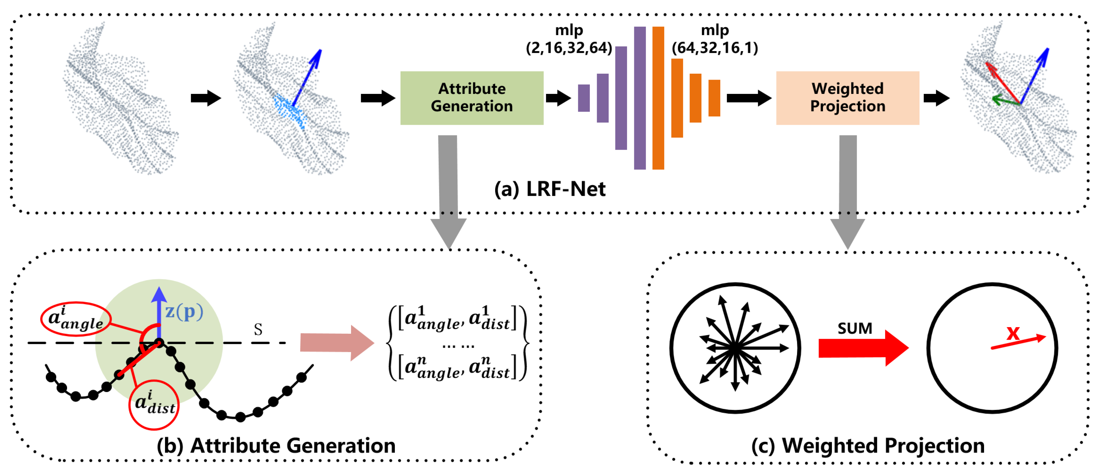
The whole architecture of LRF-Net in shown in
Figure 2a. LRF-Net predicts the direction of three axes successively. For a local surface, we first estimate its
z-axis via its normal vector computed over a small subset of the local point set. Then, unique weights are learned for each point in the local surface. The
x-axis is calculated by integrating projection vectors with learned weights using a vector-sum operation. At last, the
y-axis is calculated by the cross-product operation between
z-axis and
x-axis.
LRF definition: Given a local surface
centered at keypoint
, the LRF at
(denoted by
) can be represented as:
where
,
, and
denote the
x-axis,
y-axis, and
z-axis of
, respectively. As three axes are orthogonal, the estimation of LRF therefore contains two parts: Estimation of the
z-axis and the
x-axis.
A naive way to learn an LRF for the local surface is to train a network that directly regresses the axes. The premise is that ground-truth LRFs are labeled for local surfaces. Unfortunately, the network trained in this manner meets two difficulties. The first one is that the definition of ground-truth LRFs for local surfaces remain an open issue in the community [
8]. The second one, which is more important, is that the orthogonality of three axes cannot be guaranteed. We suggest estimating
z-axis and
x-axis independently.
Z-axis: As for
z-axis, we take the normal of the keypoint as the
z-axis., which has been confirmed [
2] to be quite repeatable. To resist the impact of clutter and occlusion, we collect a small subset of the local surface to calculate the normal. For more details, readers are referred to [
11].
X-axis: Once the
z-axis is determined, the remaining task is to compute the
x-axis. Compared with
z-axis,
x-axis is more challenging due to the influence of noise, clutter, and occlusion [
8]. We argue that each neighboring point in the local surface gives a unique contribution to LRF construction. Hence, we predict a weight for each neighboring point and leverage all neighboring points with learned weights for
x-axis prediction. The main steps are as follows.
First, to make the estimate LRF invariant to rigid transformation, our network consumes with invariant geometric attributes, rather than point coordinates. In particular, two attributes, i.e., relative distance
and surface variation angle
are used in LRF-Net as illustrated in
Figure 2b. For a neighbor
of
, the two attributes of
are computed as:
where
is the
norm and
r represents the support radius of the local surface. The range of
and
are
and
, respectively. Thus, every radius neighboring point represented by two attributes that will be encoded to a weight value via LRF-Net later. The employed two attributes in LRF-Net have two merits at least. First, the unique spatial information of a radius neighboring point in the local surface can be well represented, as shown in
Figure 3. Both attributes are complementary to each other. Second, the two attributes are calculated with respect to the keypoint, which are rotation invariant. It makes the learned weights rotation invariant as well.
Second, with geometric attributes being the input, we use a simple network with multilayer perceptions (MLP) layers only to predict weights for neighboring points. The details of the network are illustrated in
Figure 4. The network is very simple, however, is sufficient to predict stable and informative weights for neighboring points (as will be verified in the experiments).
Third, because
x-axis is orthogonal to
z-axis, we project each neighbor
on the tangent plane
of the
z-axis and compute a projection vector for
as:
We integrate all weighted projection vectors in a weighted vector-sum manner:
where
n denotes the total number of radius neighbors of keypoint
and
is a learned weight by LRF-Net. Another way for determining the
x-axis, based on these weights, is choosing the vector with the maximum weight, as in many PSD-based LRFs [
2,
10]. However, it fails to leverage all neighboring information and we will shown that it is inferior to the vector-sum operation in the experiments.
Y-axis: Based on the calculated z-axis and x-axis, the y-axis can be computed by the cross-product between them.
3.2. Weakly Supervised Training Scheme
Our training data are constituted by a series of corresponding local surface patches. The corresponding relationship is obtained based on the ground-truth rigid transformation of two whole point clouds. In particular, LRF-Net needs the corresponding relationships between local surface patches only, rather than ground-truth LRFs and/or exact pose variation information between patches. Therefore, our network can be trained in a weakly supervised manner.
We train our LRF-Net with two streams in a Siamese fashion where each stream independently predicts an LRF for a local surface. Specifically, two streams take the local surfaces of keypoints
and
as inputs, respectively. Here,
and
are two corresponding keypoints sampled from the model and scene point cloud. Both streams share the same architecture and underlying weights. We use the predicted LRFs
and
by two stream to transform the local surfaces
and
to the coordinate system of the two LRFs. Then, we calculate the Chamfer Distance [
14] between two transformed local surfaces as the loss function to train LRF-Net:
where
Our opinion is that it is difficult to define a “good” LRF for a single local surface. For 3D shape matching, LRFs that can align the poses of two local surface patches are judged as repeatable. This motivates us to consider two local patches simultaneously and employ the Chamfer Distance to train the network.


