AttPNet: Attention-Based Deep Neural Network for 3D Point Set Analysis


Abstract
1. Introduction
- We propose a novel model named AttPNet which uses attention mechanism for both global feature masking and channel weighting to focus on characteristic regions and channels.
- Our model achieved 93.6% accuracy of overall instances on ModelNet40 benchmark dataset without voting and outperforms the existing best point set model by 0.7%. Given that the performance improvement is slow in recent years, the performance improvement of our model is significant.
- Experiments show that our model generalizes better on test data with random translation, rotation, and missing points perturbations Table 1.
2. Related Work
2.1. Point Cloud Networks
2.1.1. Projection and Voxelization
2.1.2. PointNet & PointNet++
2.1.3. Graph Networks
2.1.4. Point Convolution
2.1.5. Sequence Network
2.2. Attention-Based Methods in Computer Vision
3. Method
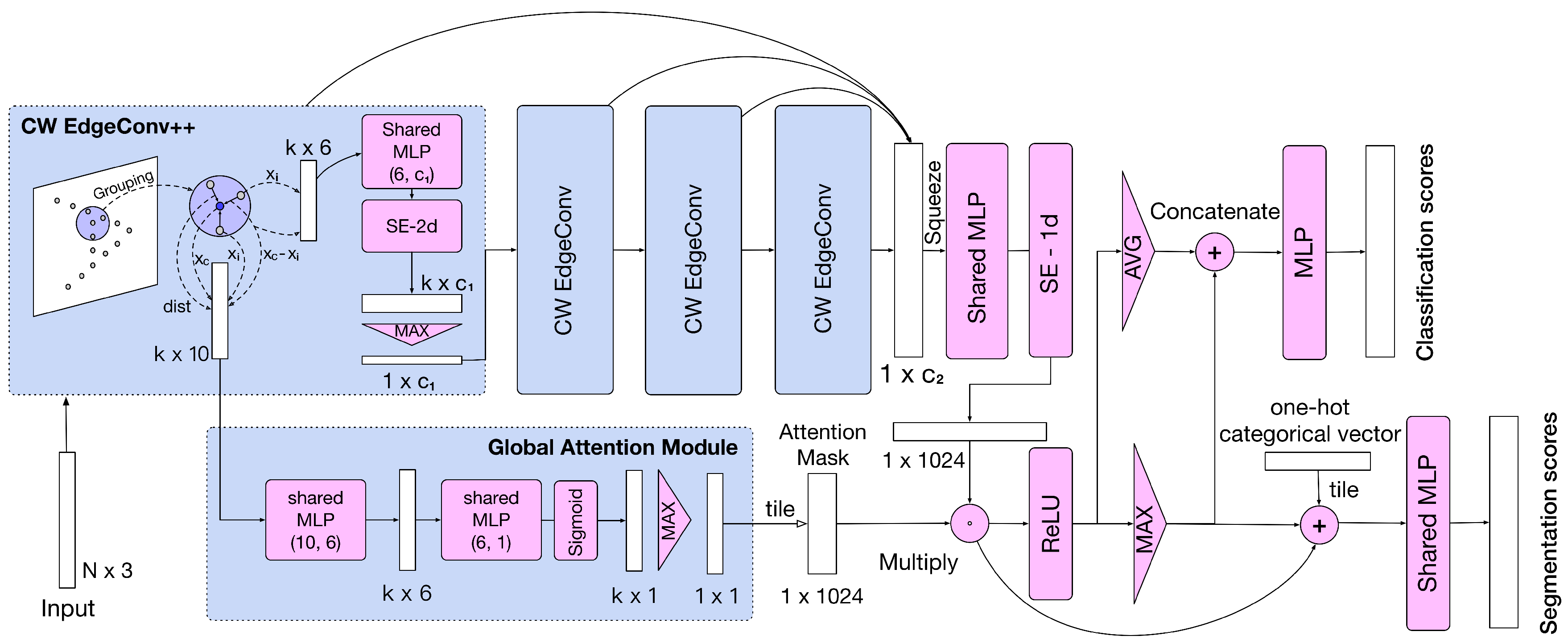
3.1. Channel Weighting Edge Convolution (CW-EdgeConv) Module
3.2. Global Attention Module
3.3. Architecture for Classification and Segmentation
3.4. Alternative Attention Modules
3.4.1. Global Hard-Attention Module
3.4.2. Spatial-Attention Edgeconv
4. Experiment
4.1. Implementation Details
4.2. Classification Results
Datasets
4.3. ModelNet40
4.4. ECT
4.5. Part Segmentation Results
4.5.1. Dataset
4.5.2. Shapenet
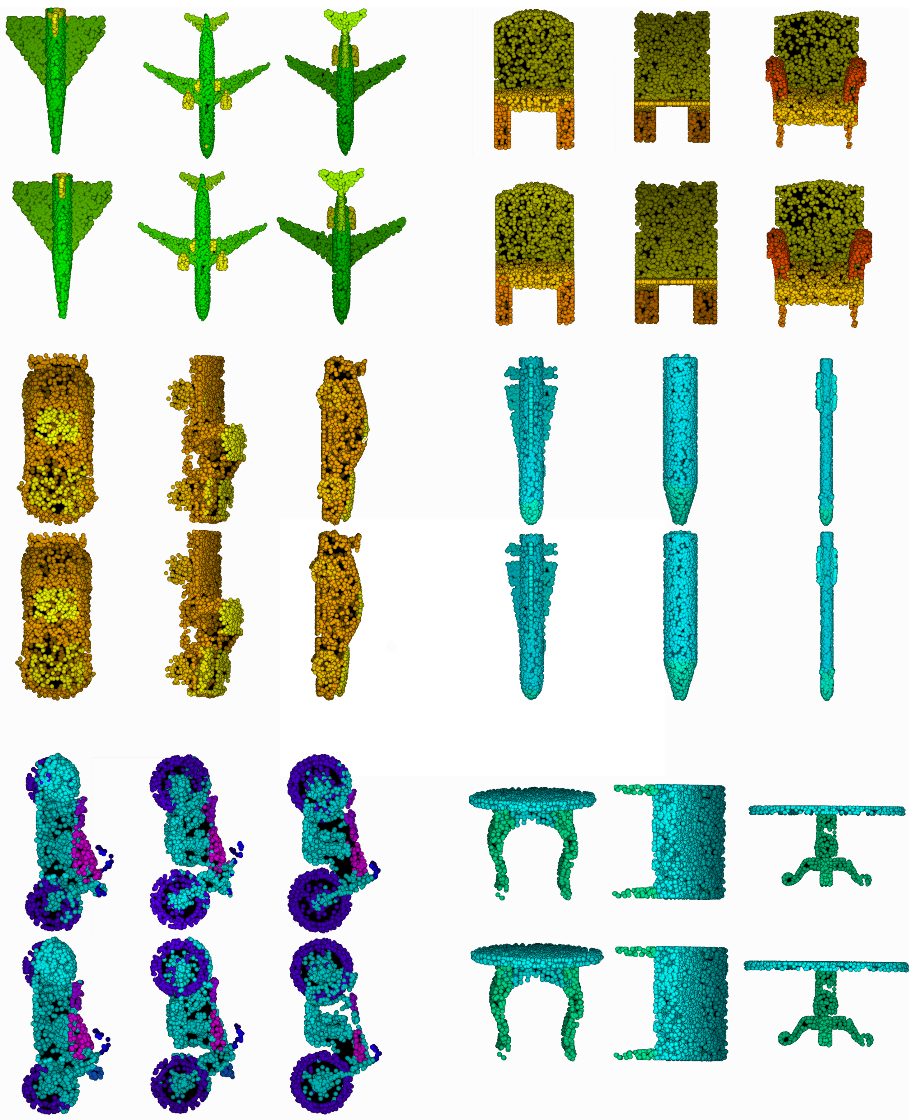
4.6. Visualization of Attention
4.7. Robustness
4.7.1. Missing Points
4.7.2. Rotation and Translation Perturbations
5. Additional Visualization of Rotated Attention Mask
6. Additional Ablation Study on the ModelNet40 Dataset
7. Conclusions
Author Contributions
Funding
Conflicts of Interest
References
- Petti, F.M.; Avanzini, M.; Belvedere, M.; De Gasperi, M.; Ferretti, P.; Girardi, S.; Remondino, F.; Tomasoni, R. Digital 3D modelling of dinosaur footprints by photogrammetry and laser scanning techniques: Integrated approach at the Coste dell’Anglone tracksite (Lower Jurassic, Southern Alps, Northern Italy). Acta Geol. 2008, 83, 303–315. [Google Scholar]
- Ahmed, E.; Saint, A.; Shabayek, A.E.R.; Cherenkova, K.; Das, R.; Gusev, G.; Aouada, D.; Ottersten, B. Deep learning advances on different 3D data representations: A survey. arXiv 2018, arXiv:1808.01462. [Google Scholar]
- Qi, C.R.; Su, H.; Mo, K.; Guibas, L.J. Pointnet: Deep learning on point sets for 3D classification and segmentation. In Proceedings of the IEEE Conference on Computer Vision and Pattern Recognition, Honolulu, HI, USA, 21–26 July 2017; pp. 652–660. [Google Scholar]
- Qi, C.R.; Yi, L.; Su, H.; Guibas, L.J. Pointnet++: Deep hierarchical feature learning on point sets in a metric space. In Advances in Neural Information Processing Systems; Curran Associates, Inc.: Long Beach, CA, USA, 2017; pp. 5099–5108. [Google Scholar]
- Hu, J.; Shen, L.; Sun, G. Squeeze-and-excitation networks. In Proceedings of the IEEE Conference on Computer Vision and Pattern Recognition, Salt Lake City, UT, USA, 18–22 June 2018; pp. 7132–7141. [Google Scholar]
- Su, H.; Maji, S.; Kalogerakis, E.; Learned-Miller, E. Multi-view convolutional neural networks for 3D shape recognition. In Proceedings of the IEEE International Conference on Computer Vision, Santiago, Chile, 7–13 December 2015; pp. 945–953. [Google Scholar]
- Qi, C.R.; Su, H.; Nießner, M.; Dai, A.; Yan, M.; Guibas, L.J. Volumetric and multi-view cnns for object classification on 3D data. In Proceedings of the IEEE Conference on Computer Vision and Pattern Recognition, Las Vegas, NV, USA, 27–30 June 2016; pp. 5648–5656. [Google Scholar]
- Lawin, F.J.; Danelljan, M.; Tosteberg, P.; Bhat, G.; Khan, F.S.; Felsberg, M. Deep projective 3D semantic segmentation. In International Conference on Computer Analysis of Images and Patterns; Springer: Berlin/Heidelberg, Germany, 2017; pp. 95–107. [Google Scholar]
- Schneider, S.; Himmelsbach, M.; Luettel, T.; Wuensche, H.J. Fusing vision and lidar-synchronization, correction and occlusion reasoning. In Proceedings of the 2010 IEEE Intelligent Vehicles Symposium, San Diego, CA, USA, 21–24 June 2010; pp. 388–393. [Google Scholar]
- Wu, Z.; Song, S.; Khosla, A.; Yu, F.; Zhang, L.; Tang, X.; Xiao, J. 3D shapenets: A deep representation for volumetric shapes. In Proceedings of the IEEE Conference on Computer Vision and Pattern Recognition, Boston, MA, USA, 7–12 June 2015; pp. 1912–1920. [Google Scholar]
- Maturana, D.; Scherer, S. Voxnet: A 3D convolutional neural network for real-time object recognition. In Proceedings of the 2015 IEEE/RSJ International Conference on Intelligent Robots and Systems (IROS), Hamburg, Germany, 28 September–2 October 2015; pp. 922–928. [Google Scholar]
- Brock, A.; Lim, T.; Ritchie, J.M.; Weston, N.J. Generative and Discriminative Voxel Modeling with Convolutional Neural Networks. In Proceedings of the Neural Inofrmation Processing Conference: 3D Deep Learning, Barcelona, Spain, 5–10 December 2016. [Google Scholar]
- Su, H.; Jampani, V.; Sun, D.; Maji, S.; Kalogerakis, E.; Yang, M.H.; Kautz, J. Splatnet: Sparse lattice networks for point cloud processing. In Proceedings of the IEEE Conference on Computer Vision and Pattern Recognition, Salt Lake City, UT, USA, 18–22 June 2018; pp. 2530–2539. [Google Scholar]
- Jampani, V.; Kiefel, M.; Gehler, P.V. Learning sparse high dimensional filters: Image filtering, dense crfs and bilateral neural networks. In Proceedings of the IEEE Conference on Computer Vision and Pattern Recognition, Las Vegas, NV, USA, 27–30 June 2016; pp. 4452–4461. [Google Scholar]
- Riegler, G.; Osman Ulusoy, A.; Geiger, A. Octnet: Learning deep 3D representations at high resolutions. In Proceedings of the IEEE Conference on Computer Vision and Pattern Recognition, Honolulu, HI, USA, 21–26 July 2017; pp. 3577–3586. [Google Scholar]
- Wang, Y.; Sun, Y.; Liu, Z.; Sarma, S.E.; Bronstein, M.M.; Solomon, J.M. Dynamic graph cnn for learning on point clouds. arXiv 2018, arXiv:1801.07829. [Google Scholar] [CrossRef]
- Shen, Y.; Feng, C.; Yang, Y.; Tian, D. Mining Point Cloud Local Structures by Kernel Correlation and Graph Pooling. In Proceedings of the IEEE Conference on Computer Vision and Pattern Recognition, Salt Lake City, UT, USA, 18–22 June 2018. [Google Scholar]
- Xu, M.; Zhou, Z.; Qiao, Y. Geometry Sharing Network for 3D Point Cloud Classification and Segmentation. In Proceedings of the National Conference on Artificial Intelligence (AAAI), New York, NY, USA, 7–12 February 2020; pp. 12500–12507. [Google Scholar]
- Wu, W.; Qi, Z.; Fuxin, L. Pointconv: Deep convolutional networks on 3D point clouds. In Proceedings of the IEEE Conference on Computer Vision and Pattern Recognition, Long Beach, CA, USA, 16–20 June 2019; pp. 9621–9630. [Google Scholar]
- Xu, Y.; Fan, T.; Xu, M.; Zeng, L.; Qiao, Y. Spidercnn: Deep learning on point sets with parameterized convolutional filters. In Proceedings of the European Conference on Computer Vision (ECCV), Munich, Germany, 8–14 September 2018; pp. 87–102. [Google Scholar]
- Groh, F.; Wieschollek, P.; Lensch, H.P. Flex-Convolution. In Proceedings of the Asian Conference on Computer Vision, Perth, Australia, 2–6 December 2018; pp. 105–122. [Google Scholar]
- Wang, L.; Liu, Y.; Zhang, S.; Yan, J.; Tao, P. Structure-Aware Convolution for 3D Point Cloud Classification and Segmentation. Remote Sens. 2020, 12, 634. [Google Scholar] [CrossRef]
- Liu, X.; Han, Z.; Liu, Y.S.; Zwicker, M. Point2Sequence: Learning the shape representation of 3D point clouds with an attention-based sequence to sequence network. In Proceedings of the AAAI Conference on Artificial Intelligence, Honolulu, HI, USA, 27 January–1 February 2019; Volume 33, pp. 8778–8785. [Google Scholar]
- Hochreiter, S.; Schmidhuber, J. Long short-term memory. Neural Comput. 1997, 9, 1735–1780. [Google Scholar] [CrossRef] [PubMed]
- Itti, L. A model of saliency-based visual attention for rapid scene analysis. IEEE Trans. 1998, 20, 1254–1259. [Google Scholar] [CrossRef]
- Bahdanau, D.; Cho, K.; Bengio, Y. Neural machine translation by jointly learning to align and translate. arXiv 2014, arXiv:1409.0473. [Google Scholar]
- Fu, J.; Zheng, H.; Mei, T. Look closer to see better: Recurrent attention convolutional neural network for fine-grained image recognition. In Proceedings of the IEEE Conference on Computer Vision and Pattern Recognition, Honolulu, HI, USA, 21–26 July 2017; pp. 4438–4446. [Google Scholar]
- Wang, F.; Jiang, M.; Qian, C.; Yang, S.; Li, C.; Zhang, H.; Wang, X.; Tang, X. Residual attention network for image classification. In Proceedings of the IEEE Conference on Computer Vision and Pattern Recognition, Honolulu, HI, USA, 21–26 July 2017; pp. 3156–3164. [Google Scholar]
- Chen, L.C.; Yang, Y.; Wang, J.; Xu, W.; Yuille, A.L. Attention to scale: Scale-aware semantic image segmentation. In Proceedings of the IEEE Conference on Computer Vision and Pattern Recognition, Las Vegas, NV, USA, 27–30 June 2016; pp. 3640–3649. [Google Scholar]
- Xie, S.; Liu, S.; Chen, Z.; Tu, Z. Attentional ShapeContextNet for Point Cloud Recognition. In Proceedings of the 2018 IEEE/CVF Conference on Computer Vision and Pattern Recognition, Salt Lake City, UT, USA, 18–22 June 2018; pp. 4606–4615. [Google Scholar] [CrossRef]
- Yang, J.; Zhang, Q.; Ni, B.; Li, L.; Liu, J.; Zhou, M.; Tian, Q. Modeling Point Clouds with Self-Attention and Gumbel Subset Sampling. In Proceedings of the 2018 IEEE/CVF Conference on Computer Vision and Pattern Recognition, Long Beach, CA, USA, 16–20 June 2019; pp. 3323–3332. [Google Scholar]
- Li, W.; Wang, F.D.; Xia, G.S. A geometry-attentional network for ALS point cloud classification. ISPRS J. Photogramm. Remote Sens. 2020, 164, 26–40. [Google Scholar] [CrossRef]
- Hu, Z.; Zhang, D.; Li, S.; Qin, H. Attention-based relation and context modeling for point cloud semantic segmentation. Comput. Graph. 2020. [Google Scholar] [CrossRef]
- Wang, L.; Huang, Y.; Hou, Y.; Zhang, S.; Shan, J. Graph Attention Convolution for Point Cloud Semantic Segmentation. In Proceedings of the IEEE Conference on Computer Vision and Pattern Recognition, Long Beach, CA, USA, 16–20 June 2019; pp. 10296–10305. [Google Scholar]
- Hastie, T.; Tibshirani, R.; Friedman, J.; Franklin, J. The elements of statistical learning: Data mining, inference and prediction. Math. Intell. 2005, 27, 83–85. [Google Scholar]
- Ioffe, S.; Szegedy, C. Batch Normalization: Accelerating Deep Network Training by Reducing Internal Covariate Shift. In Proceedings of the International Conference on Machine Learning, Lille, France, 6 July 2015; pp. 448–456. [Google Scholar]
- Nair, V.; Hinton, G.E. Rectified linear units improve restricted boltzmann machines. In Proceedings of the 27th International Conference on Machine Learning (ICML-10), Haifa, Israel, 21–24 June 2010; pp. 807–814. [Google Scholar]
- Li, Y.; Bu, R.; Sun, M.; Wu, W.; Di, X.; Chen, B. Pointcnn: Convolution on x-transformed points. In Proceedings of the Advances in Neural Information Processing Systems, Montréal, QC, Canada, 3–8 December 2018; pp. 820–830. [Google Scholar]
- Atzmon, M.; Maron, H.; Lipman, Y. Point convolutional neural networks by extension operators. arXiv 2018, arXiv:1803.10091. [Google Scholar] [CrossRef]
- Liu, Y.; Fan, B.; Xiang, S.; Pan, C. Relation-Shape Convolutional Neural Network for Point Cloud Analysis. In Proceedings of the IEEE Conference on Computer Vision and Pattern Recognition, Long Beach, CA, USA, 16–20 June 2019; pp. 8895–8904. [Google Scholar]
- Li, J.; Chen, B.M.; Hee Lee, G. So-net: Self-organizing network for point cloud analysis. In Proceedings of the IEEE Conference on Computer Vision and Pattern Recognition, Salt Lake City, UT, USA, 18–22 June 2018; pp. 9397–9406. [Google Scholar]
- Loshchilov, I.; Hutter, F. Sgdr: Stochastic gradient descent with warm restarts. arXiv 2016, arXiv:1608.03983. [Google Scholar]
- Noble, A.J.; Dandey, V.P.; Wei, H.; Brasch, J.; Chase, J.; Acharya, P.; Tan, Y.Z.; Zhang, Z.; Kim, L.Y.; Scapin, G.; et al. Routine single particle CryoEM sample and grid characterization by tomography. Elife 2018, 7, e34257. [Google Scholar] [CrossRef] [PubMed]
- Yi, L.; Su, H.; Guo, X.; Guibas, L. SyncSpecCNN: Synchronized Spectral CNN for 3D Shape Segmentation. In Proceedings of the IEEE Conference on Computer Vision and Pattern Recognition, Honolulu, HI, USA, 21–26 July 2017; pp. 9397–9406. [Google Scholar]


| Method | Translation | R | R | R |
|---|---|---|---|---|
| Ours | 93.4 | 93.2 | 92.1 | 86.3 |
| PointNet++ | 90.6 | 90.3 | 88.6 | 83.8 |
| Method | Input | OA (%) |
|---|---|---|
| PointNet [3] | 1024 | 89.2 |
| PointNet++ [4] | 1024 | 90.7 |
| PointNet++ [4] | 5000 + n | 91.9 |
| PointCNN [38] | 1024 | 92.2 |
| DGCNN [16] | 1024 | 92.2 |
| PCNN [39] | 1024 | 92.3 |
| SpiderCNN [20] | 1024 + n | 92.2 |
| SpiderCNN-4 [20] | 1024 + n | 92.4 |
| PointConv [19] | 1024 + n | 92.5 |
| Point2seq [23] | 1024 | 92.6 |
| RS-CNN [40] | 1024 | 92.9 |
| SO-Net-2 [41] | 2048 | 90.9 |
| SO-Net-3 [41] | 5000 + n | 93.4 |
| Ours (BASELINE) | 1024 | 92.5 |
| Ours (global attention) | 1024 | 92.9 |
| Ours (hard attention) | 1024 | 92.5 |
| Ours (multi-attention) | 1024 | 93.3 |
| Ours (global + channel) | 1024 | 93.6 |
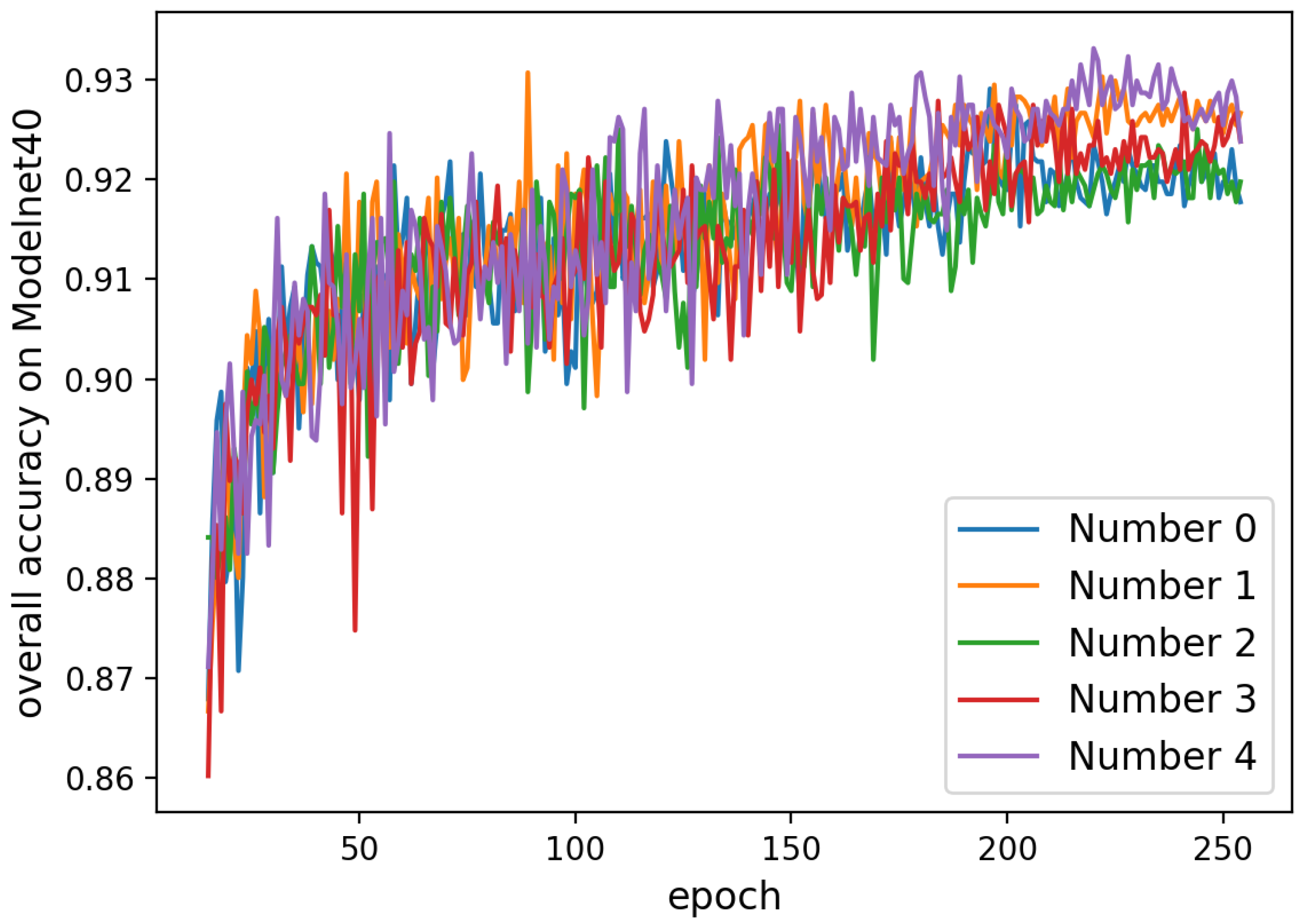
| Number | 0 | 1 | 2 | 3 | 4 |
|---|---|---|---|---|---|
| OA (%) | 92.8 | 93.1 | 92.6 | 92.9 | 93.3 |
| Method | OA (%) |
|---|---|
| PointNet [3] | 47.78 |
| PointNet++ [4] | 94.62 |
| Ours (global + channel) | 96.28 |
| Method | Class mIoU | Instance mIoU |
|---|---|---|
| PointNet [3] | 80.4 | 83.7 |
| PointNet++ * [4] | 81.9 | 85.1 |
| SpiderCNN [20] | 82.4 | 85.3 |
| SPLATNet [13] | 82.0 | 84.6 |
| SyncSpecCNN [44] | 82.0 | 84.7 |
| DGCNN [16] | 82.3 | 85.1 |
| SO-Net * [41] | 80.8 | 84.6 |
| Ours | 82.8 | 85.2 |
| Model | #Points | BN | DP | Act. | Max | Max&Avg. | Acc |
|---|---|---|---|---|---|---|---|
| A1 | 1 k | LR | √ | 90.8 | |||
| A2 | 1 k | √ | LR | √ | 91.6 | ||
| A3 | 1 k | √ | LR | √ | 93.2 | ||
| A4 | 1 k | √ | √ | LR | √ | 93.6 | |
| A5 | 1 k | √ | √ | R | √ | 92.8 | |
| A6 | 2 k | √ | √ | LR | √ | 93.6 | |
| A7 | 1 k | √ | √ | LR | √ | 93.3 |
© 2020 by the authors. Licensee MDPI, Basel, Switzerland. This article is an open access article distributed under the terms and conditions of the Creative Commons Attribution (CC BY) license (http://creativecommons.org/licenses/by/4.0/).
Share and Cite
Yang, Y.; Ma, Y.; Zhang, J.; Gao, X.; Xu, M. AttPNet: Attention-Based Deep Neural Network for 3D Point Set Analysis. Sensors 2020, 20, 5455. https://doi.org/10.3390/s20195455
Yang Y, Ma Y, Zhang J, Gao X, Xu M. AttPNet: Attention-Based Deep Neural Network for 3D Point Set Analysis. Sensors. 2020; 20(19):5455. https://doi.org/10.3390/s20195455
Chicago/Turabian StyleYang, Yufeng, Yixiao Ma, Jing Zhang, Xin Gao, and Min Xu. 2020. "AttPNet: Attention-Based Deep Neural Network for 3D Point Set Analysis" Sensors 20, no. 19: 5455. https://doi.org/10.3390/s20195455
APA StyleYang, Y., Ma, Y., Zhang, J., Gao, X., & Xu, M. (2020). AttPNet: Attention-Based Deep Neural Network for 3D Point Set Analysis. Sensors, 20(19), 5455. https://doi.org/10.3390/s20195455