Network Optimisation and Performance Analysis of a Multistatic Acoustic Navigation Sensor †


Abstract
1. Introduction
2. Sound Attenuation
3. Acoustic Positioning and Navigation System
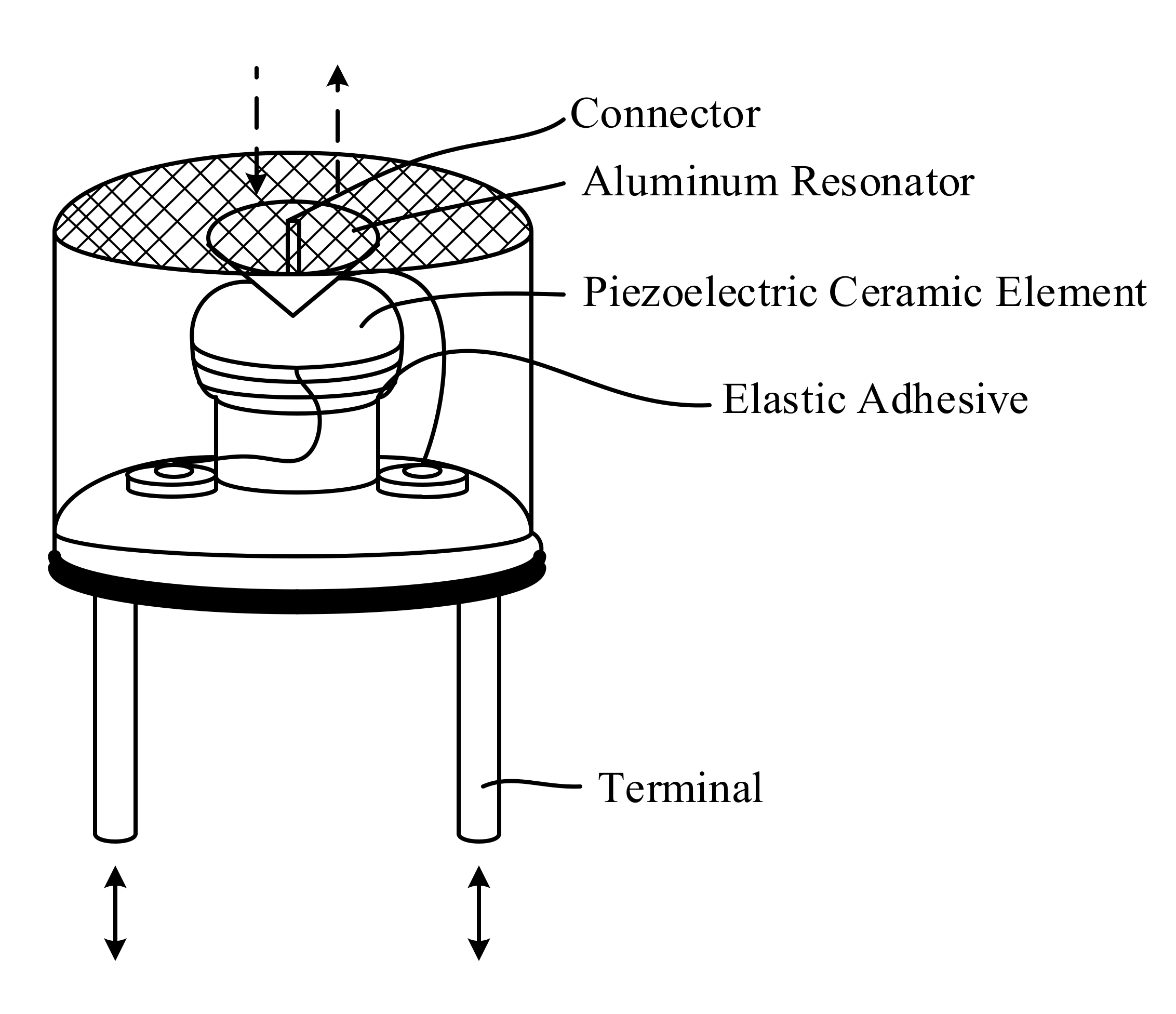
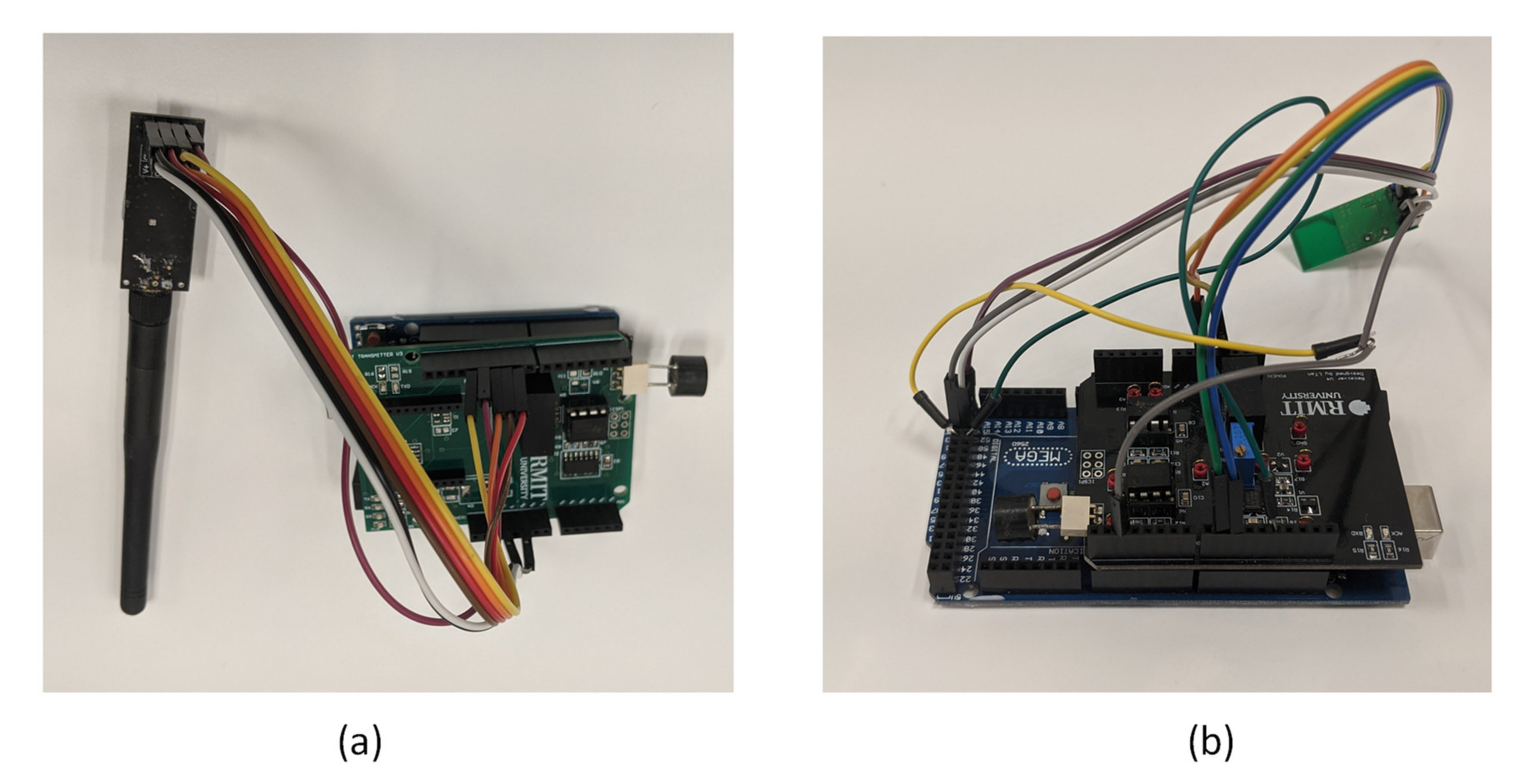
3.1. Ultrasonic Transducer
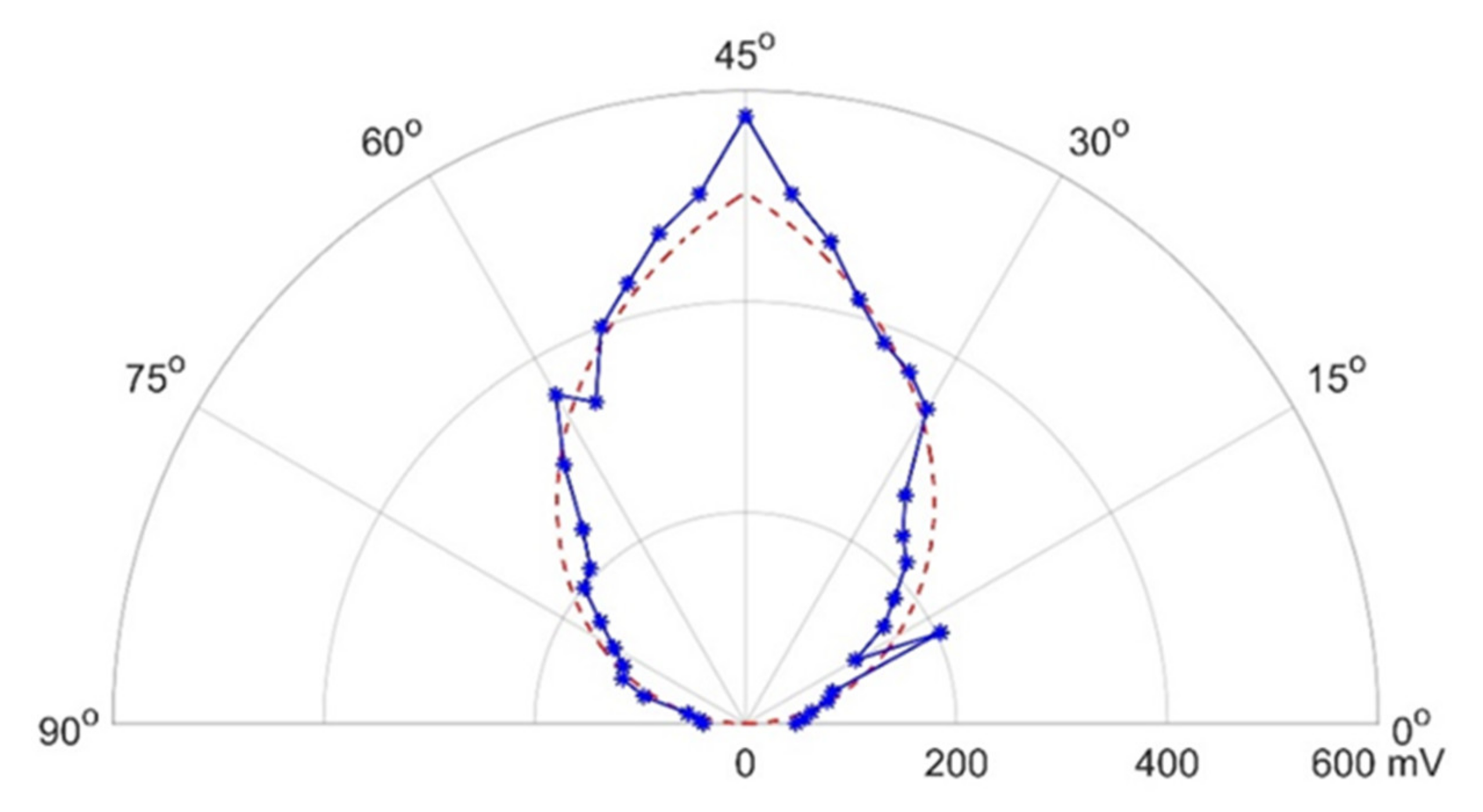
3.2. APNS Characterisation
4. Error Sources in APNS
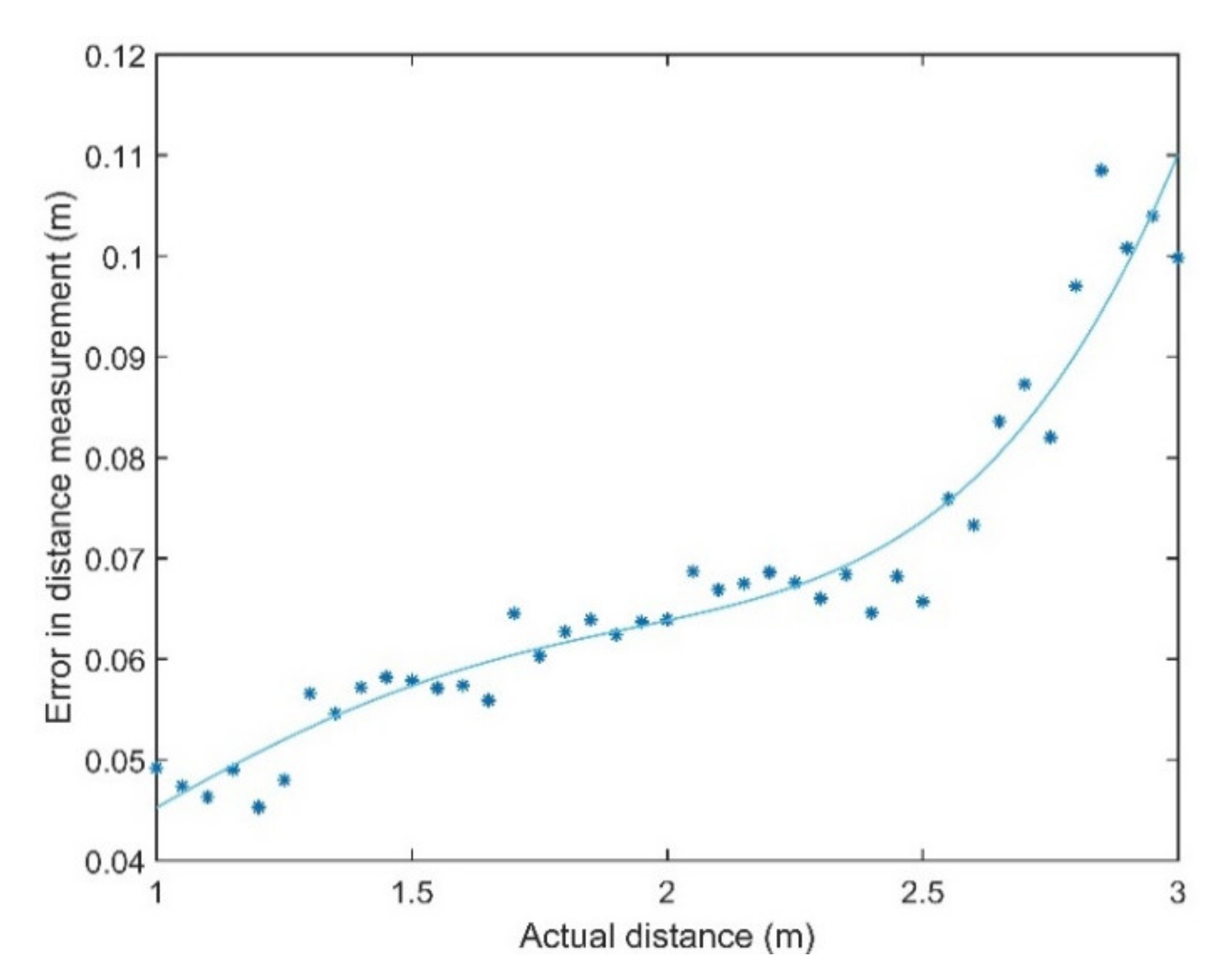
4.1. Propagation Error
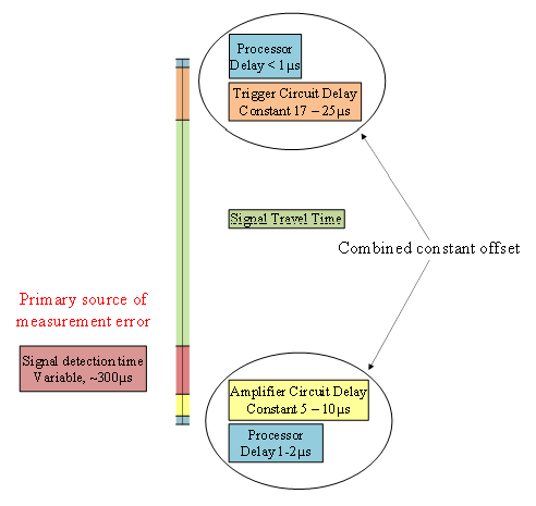
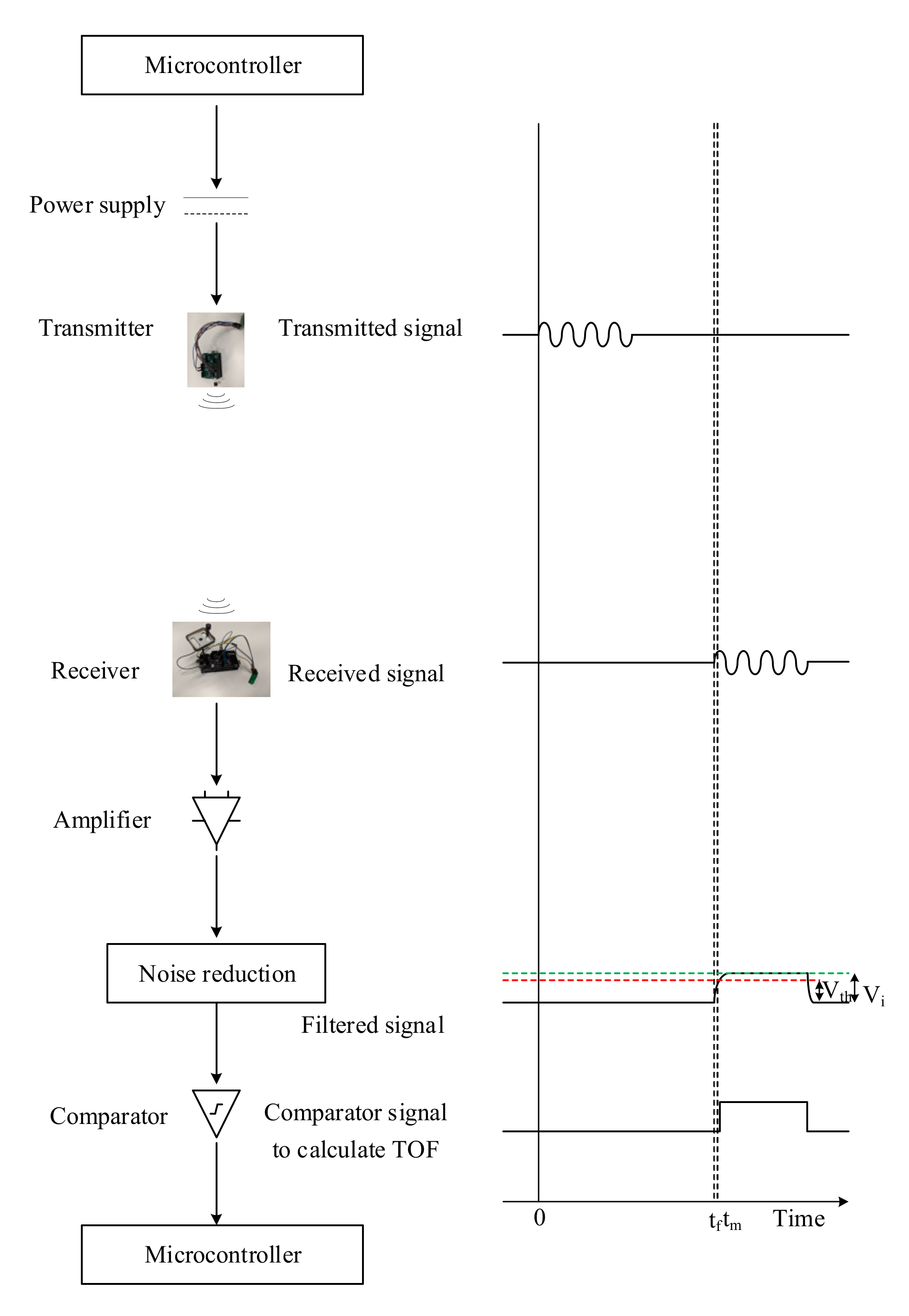
4.2. Hardware Delays
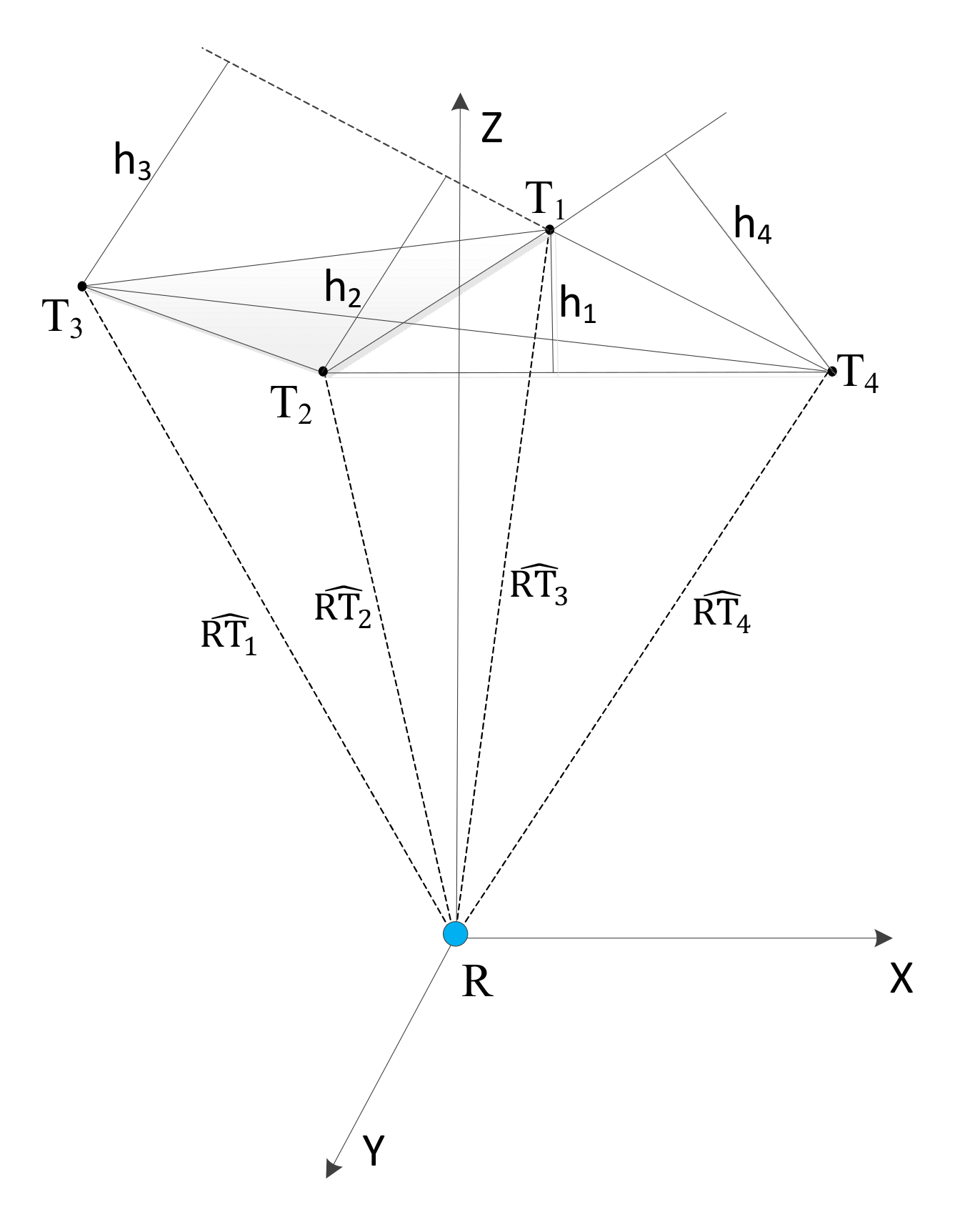
4.3. Navigation Error
5. Results
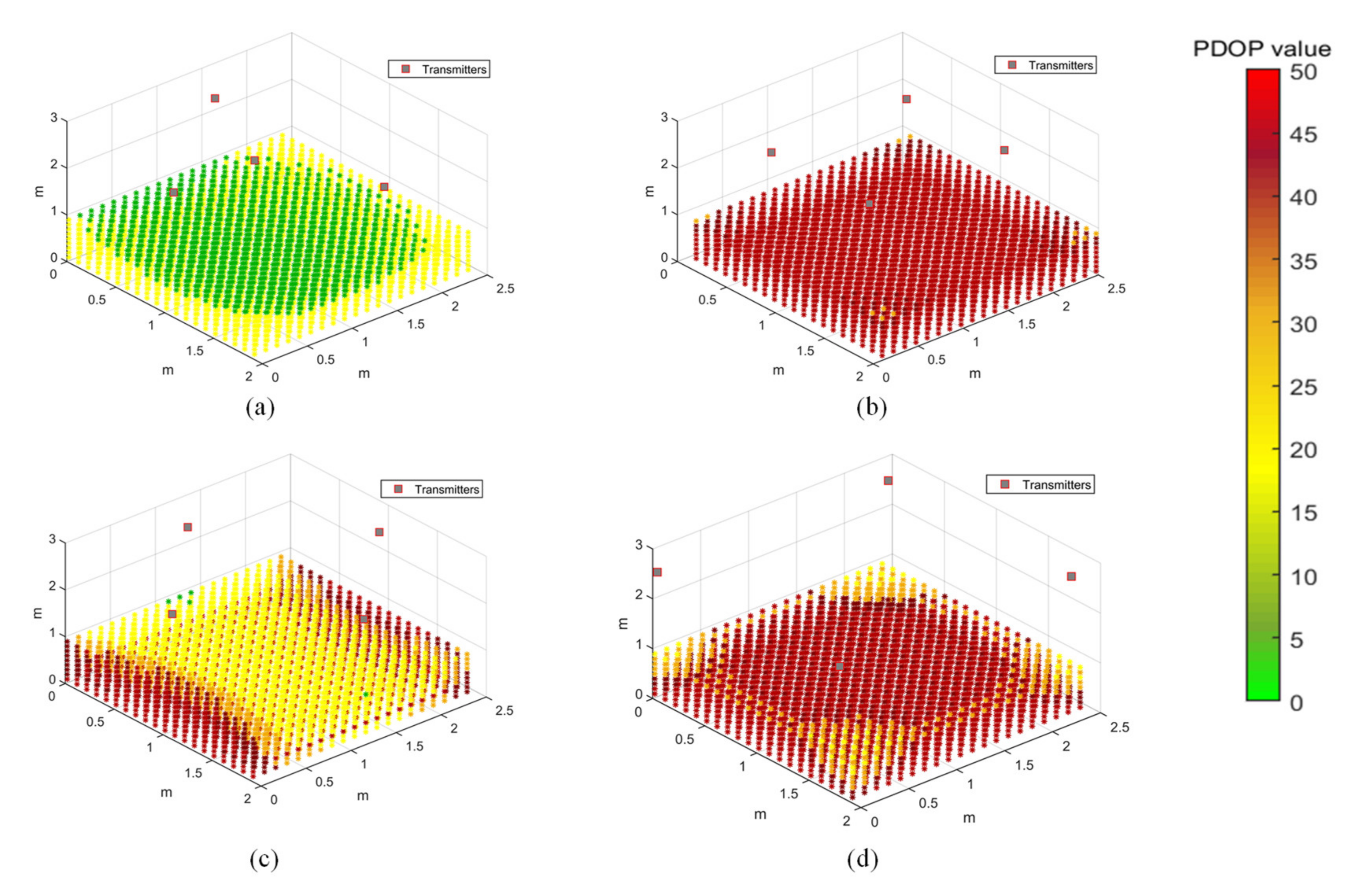
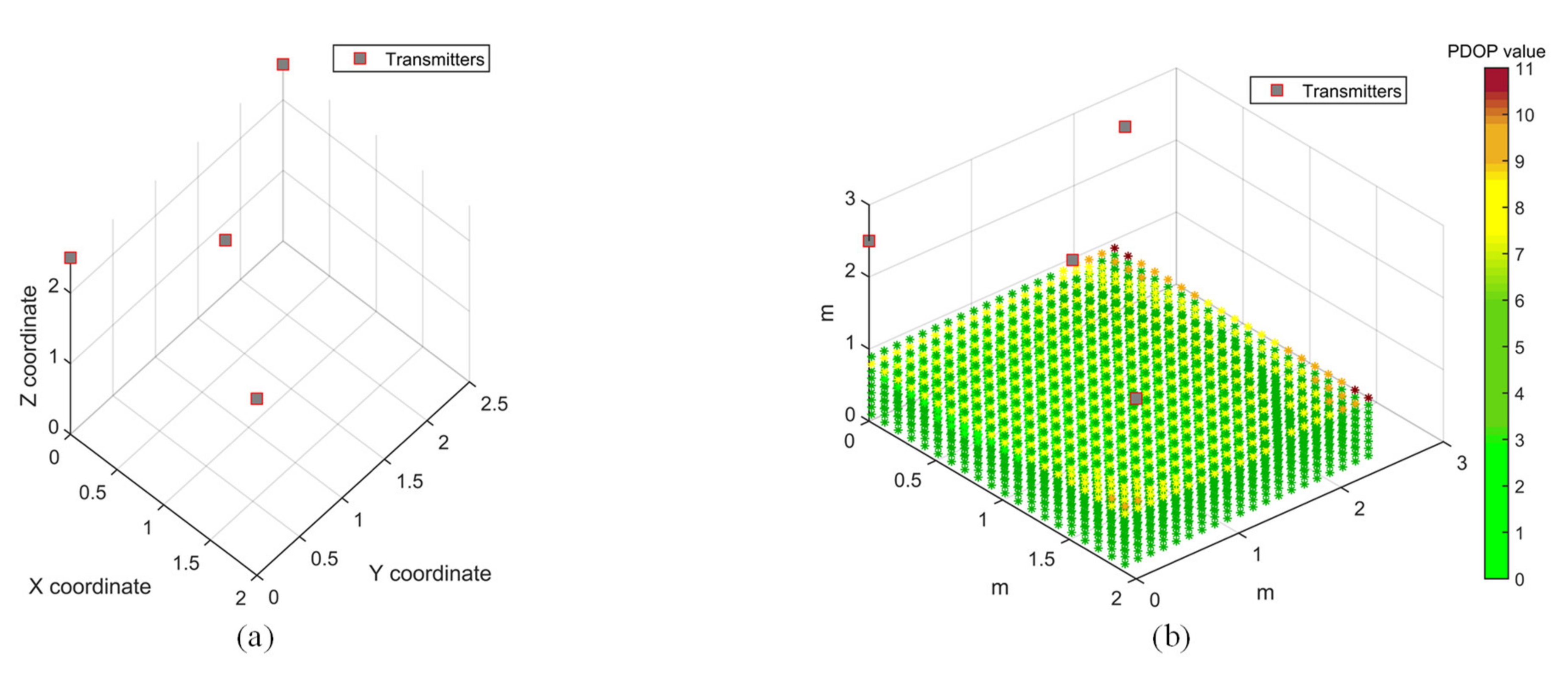
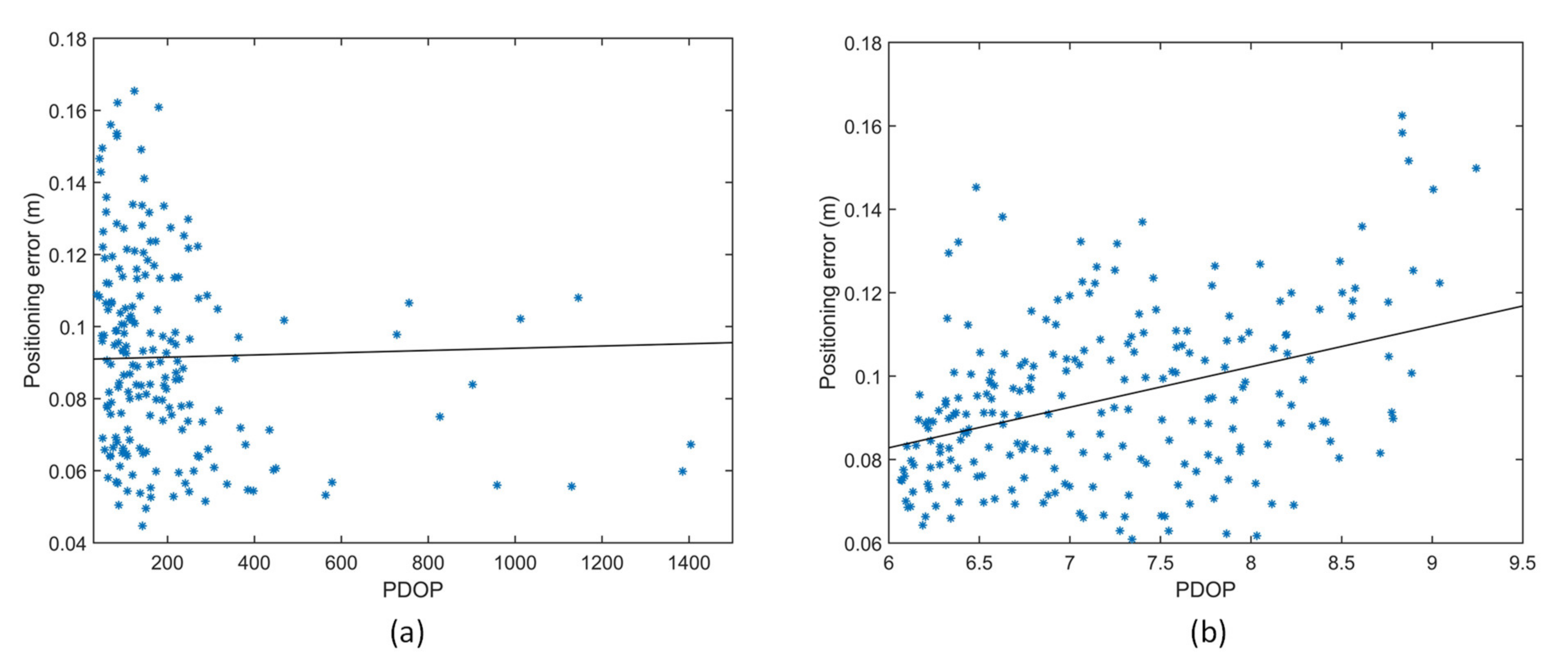
5.1. PDOP Optimisation Case Study
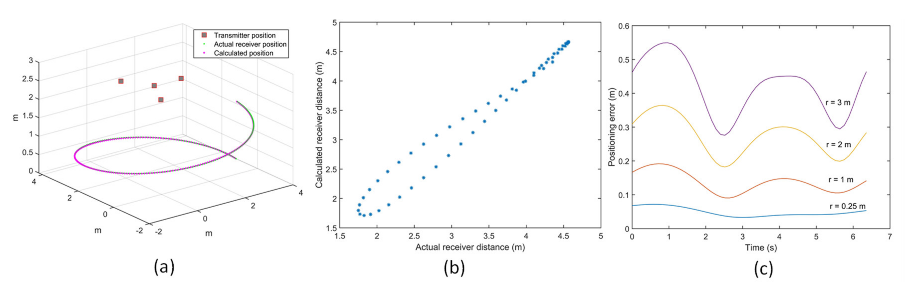
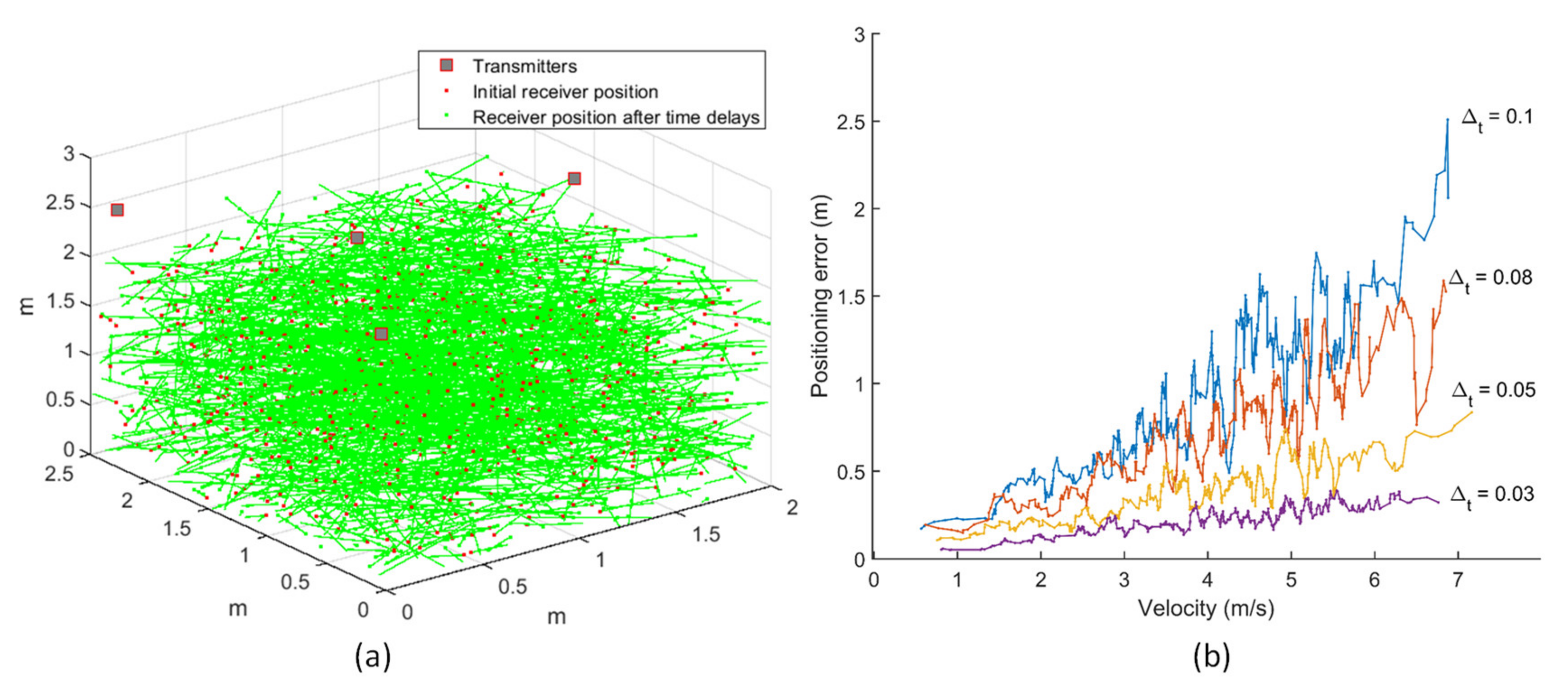
5.2. Receiver Motion Simulation
5.3. Error Budgeting
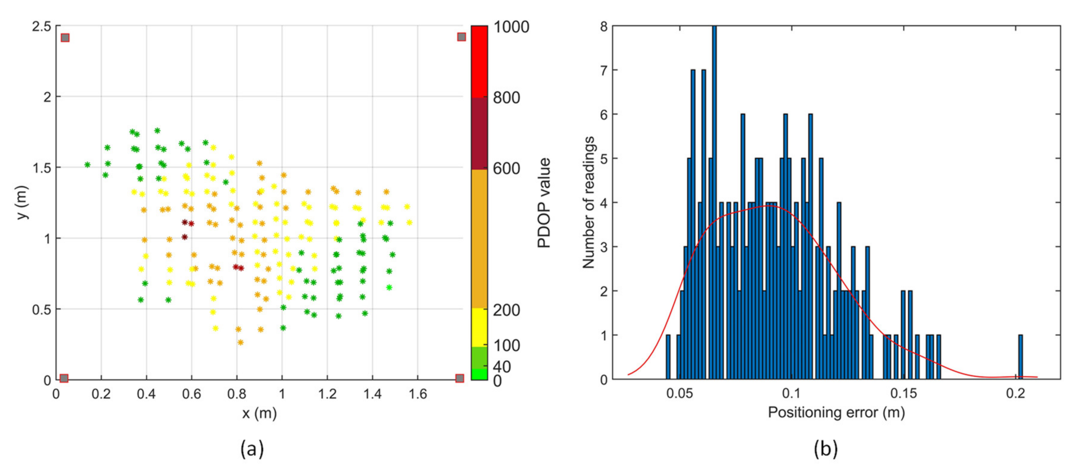
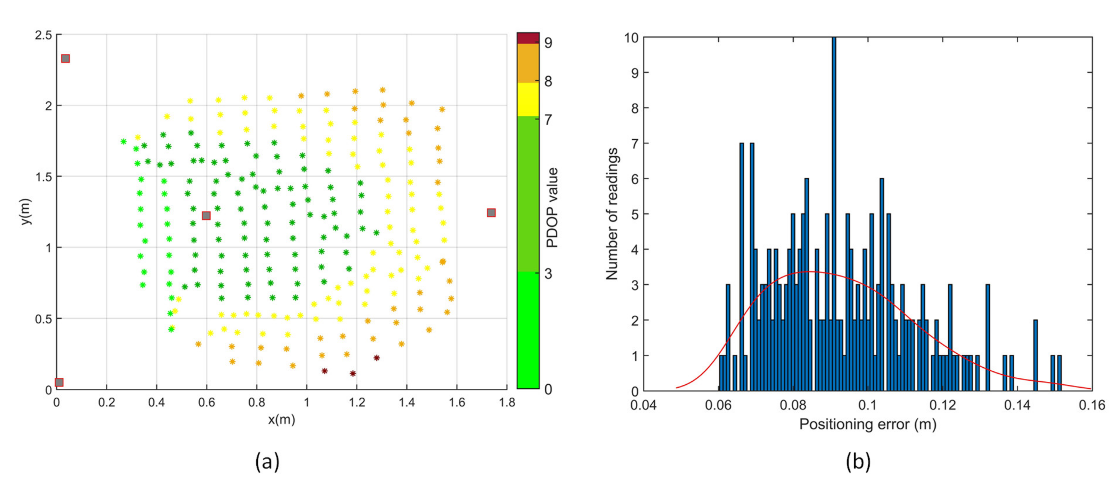
5.4. Positioning Tests
6. Conclusions
Author Contributions
Funding
Conflicts of Interest
References
- Ureña, J.; Hernández, Á.; García, J.J.; Villadangos, J.M.; Pérez, M.C.; Gualda, D.; Alvarez, F.J.; Aguilera, T. Acoustic Local Positioning with Encoded Emission Beacons. Proc. IEEE 2018, 106, 1042–1062. [Google Scholar] [CrossRef]
- Mautz, R. Indoor Positioning Technologies; ETH Zurich, Department of Civil, Environmental and Geomatic Engineering, Institute of Geodesy and Photogrammetry: Zurich, Switzerland, 2012. [Google Scholar]
- Qualisys Motion Capture System. Available online: www.qualisys.com (accessed on 23 April 2020).
- Fluerasu, A.; Vervisch-Picois, A.; Boiero, G.; Ghinamo, G.; Lovisolo, P.; Samama, N. Indoor positioning using GPS transmitters: Experimental results. In Proceedings of the 2010 International Conference on Indoor Positioning and Indoor Navigation, Zurich, Switzerland, 15–17 September 2010; pp. 1–9. [Google Scholar]
- Rizos, C.; Li, Y.; Politi, N.; Barnes, J.; Gambale, N. Locata: A new constellation for high accuracy outdoor and indoor positioning. In Proceedings of the FIG Working Week, Marrakech, Morocco, 18–22 May 2011. [Google Scholar]
- Scannapieco, A.F.; Renga, A.; Moccia, A. Compact millimeter wave FMCW InSAR for UAS indoor navigation. In Proceedings of the IEEE International Workshop on Metrology for Aerospace, Benevento, Italy, 4–5 June 2015; pp. 551–556. [Google Scholar]
- Brzozowski, B.; Kaźmierczak, K. Magnetic field mapping as a support for UAV indoor navigation system. In Proceedings of the IEEE International Workshop on Metrology for AeroSpace (MetroAeroSpace), Padua, Italy, 21–23 June 2017; pp. 583–588. [Google Scholar]
- Shen, S.; Michael, N.; Kumar, V. Autonomous multi-floor indoor navigation with a computationally constrained MAV. In Proceedings of the IEEE International Conference on Robotics and Automation (ICRA), Shanghai, China, 9–13 May 2011; pp. 20–25. [Google Scholar]
- Kulyukin, V.; Gharpure, C.; Nicholson, J.; Pavithran, S. RFID in robot-assisted indoor navigation for the visually impaired. In Proceedings of the IEEE/RSJ International Conference on Intelligent Robots and Systems (IROS)—Cover, Sendai, Japan, 28 September–2 October 2004; Volume 2, pp. 1979–1984. [Google Scholar]
- Priyantha, N.B.; Chakraborty, A.; Balakrishnan, H. The cricket location-support system. In Proceedings of the 6th annual International Conference on Mobile Computing and Networking, Boston, MA USA, 6–11 August 2000; pp. 32–43. [Google Scholar]
- Hexamite. Available online: https://www.hexamite.com/ (accessed on 6 March 2020).
- Marvelmind Robotics. Available online: https://www.marvelmind.com/ (accessed on 6 March 2020).
- Kapoor, R.; Ramasamy, S.; Gardi, A.; Schyndel, R.V.; Sabatini, R. Acoustic sensors for air and surface navigation applications. Sensors 2018, 18, 499. [Google Scholar] [CrossRef] [PubMed]
- Attenborough, K. Sound propagation in the atmosphere. In Handbook of Acoustics; Springer: Berlin, Germany, 2014; pp. 117–155. [Google Scholar]
- International Organization for Standardization. ISO 9613-1: 1993, Acoustics: Attenuation of Sound During Propagation Outdors. Caldulation of the Absorption of Sound by the Atmosphere; International Organization for Standardization: Geneva, Switzerland, 1993. [Google Scholar]
- Norma, I. 9613–2: Acoustic Attenuation of Sound during Propagation Outdoors–General Methods of Calculation; International Standard: Geneva, Switzerland, 1996. [Google Scholar]
- Wong, G.S. Approximate equations for some acoustical and thermodynamic properties of standard air. J. Acoust. Soc. Jpn. 1990, 11, 145–155. [Google Scholar] [CrossRef]
- Wong, G.S. Microphones and Their Calibration. In Handbook of Acoustics; Springer: Berlin, Germany, 2014; pp. 1061–1091. [Google Scholar]
- Wong, G.S. Speed of sound in standard air. J. Acoust. Soc. Am. 1986, 79, 1359–1366. [Google Scholar] [CrossRef]
- Wong, G.S.; Embleton, T.F.; Ehrlich, S.L. Primary pressure calibration by reciprocity. In: AIP Handbook of Condenser Microphones (Theory, Calibration, and Measurements). Acoust. Soc. Am. J. 1995, 98, 99. [Google Scholar]
- Matsushita Electronic Company Ultrasonic Ceramic Microphone Data Sheet. Available online: https://www.jameco.com/Jameco/Products/ProdDS/2120268.pdf (accessed on 1 June 2020).
- Kapoor, R.; Ramasamy, S.; Gardi, A.; Bieber, C.; Silverberg, L.; Sabatini, R. A novel 3D multilateration sensor using distributed ultrasonic beacons for indoor navigation. Sensors 2016, 16, 1637. [Google Scholar] [CrossRef] [PubMed]
- Fujieda, N.; Shinohara, T.; Ichikawa, S.; Sakaguchi, Y.; Matsuoka, S.; Kawaguchi, H. Attenuation Model for Error Correction of Ultrasonic Positioning System. IEEJ J. Ind. Appl. 2018, 7, 181–188. [Google Scholar] [CrossRef]
- Kapoor, R.; Gardi, A.G.; Sabatini, R. A Multistatic Ultrasonic Navigation System for GNSS-denied Environments. In Proceedings of the AIAA Science and Technology Forum and Exposition (SciTech), San Diego, CA, USA, 7–11 January 2019; p. 930. [Google Scholar]
- Kayton, M.; Fried, W.R. Avionics Navigation Systems; John Wiley & Sons: Hoboken, NJ, USA, 1997. [Google Scholar]
- Sabatini, R.; Moore, T.; Ramasamy, S. Global navigation satellite systems performance analysis and augmentation strategies in aviation. Prog. Aerosp. Sci. 2017. [Google Scholar] [CrossRef]
- Phillips, A.H. Geometrical determination of PDOP. Navigation 1984, 31, 329–337. [Google Scholar] [CrossRef]
- Roa, O.; Jiménez, A.R.; Seco, F.; Prieto, J.C.; Ealo, J. Optimal placement of sensors for trilateration: Regular lattices vs meta-heuristic solutions. In Proceedings of the 11th International Conference on Computer Aided Systems Theory, Las Palmas de Gran Canaria, Spain, 12–16 February 2007; pp. 780–787. [Google Scholar]


| Coefficient Constants | Value | Unit |
|---|---|---|
| a0 | 1.000100 | - |
| a1 | 1.8286 × 10⁻³ | °C−1 |
| a2 | −1.6925 × 10⁻⁶ | °C−2 |
| a3 | −3.1066 × 10⁻³ | - |
| a4 | −7.9762 × 10⁻⁶ | °C−1 |
| a5 | 3.4000 × 10⁻⁹ | °C−2 |
| a6 | 8.9180 × 10⁻⁴ | - |
| a7 | 7.7893 × 10⁻⁵ | °C−1 |
| a8 | 1.3795 × 10⁻⁶ | °C−2 |
| a9 | 9.5330 × 10⁻⁸ | °C−3 |
| a10 | 1.2990 × 10⁻⁵ | - |
| a11 | 4.8016 × 10⁻⁵ | - |
| a12 | −1.4660 × 10⁻⁶ | °C−1 |
| Parameter | Value | Unit |
|---|---|---|
| Operating temperature range | −40 to 85 | °C |
| Capacitance | 2550 | pF |
| Sensitivity | −63 | dB typically (0 dB = 10 V/Pa) |
| Directivity | 80 (typically) | degrees |
| Centre frequency | 40 | kHz |
| Capacitance tolerance | ±20 | % |
| Type | Parameters |
|---|---|
| Measured observables | Range, velocity, azimuth, and elevation |
| Environmental parameters | Temperature, wind, humidity, and environmental layout |
| Design parameters | Transmitted power, carrier frequency, and pulse repetition frequency (PRF) |
| Performance indicators | Ranging accuracy and resolution |
| Variable | Value | Unit |
|---|---|---|
| Time of flight (t) | 0.00879 | s |
| Speed of sound at sea level (c0) | 340.27 | m/s |
| Direction of receiver motion to the LOS (θ) | 56.31 | deg |
| Mach number for the sound source (M) | 0.0029 | - |
| Speed of sound emitted by source (c) at 20 °C | 345 | m/s |
| Variation of temperature with height (λ) | −0.0065 | K/m |
| Distance between ith transmitter and reflection point () | 9.98 | m |
| Distance between ith transmitter and receiver () | 10 | m |
| Distance between ith receiver and reflection point () | 0.02 | m |
| Sea-level temperature (T0) | 288 | K |
| Horizontal wind velocity (vw) | 2.95 | m/s |
| Angle of wave front normal with the horizontal (δ) | 60 | deg |
| Error Source | 1-Sigma Error (cm) |
|---|---|
| Estimated positioning error | 0.8 |
| Circuit delays | 0.1 |
| Doppler effect (velocity 3 m/s) | 0.2 |
| Receiver motion (velocity 3 m/s) | 8.2 |
| Total estimated error | 9.3 |
| Transmitter Arrangement | Mean Positioning Error (cm) | 1-sigma Positioning Error (cm) | Maximum PDOP | Minimum PDOP | Coverage (%) |
|---|---|---|---|---|---|
| Rectangular | 9.2 | 2.8 | >>99 | 37.67 | 35.35 |
| Trigonal planar | 9.5 | 2.0 | 9.24 | 6.06 | 81.78 |
© 2020 by the authors. Licensee MDPI, Basel, Switzerland. This article is an open access article distributed under the terms and conditions of the Creative Commons Attribution (CC BY) license (http://creativecommons.org/licenses/by/4.0/).
Share and Cite
Kapoor, R.; Gardi, A.; Sabatini, R. Network Optimisation and Performance Analysis of a Multistatic Acoustic Navigation Sensor. Sensors 2020, 20, 5718. https://doi.org/10.3390/s20195718
Kapoor R, Gardi A, Sabatini R. Network Optimisation and Performance Analysis of a Multistatic Acoustic Navigation Sensor. Sensors. 2020; 20(19):5718. https://doi.org/10.3390/s20195718
Chicago/Turabian StyleKapoor, Rohan, Alessandro Gardi, and Roberto Sabatini. 2020. "Network Optimisation and Performance Analysis of a Multistatic Acoustic Navigation Sensor" Sensors 20, no. 19: 5718. https://doi.org/10.3390/s20195718
APA StyleKapoor, R., Gardi, A., & Sabatini, R. (2020). Network Optimisation and Performance Analysis of a Multistatic Acoustic Navigation Sensor. Sensors, 20(19), 5718. https://doi.org/10.3390/s20195718