Ball Tracking and Trajectory Prediction for Table-Tennis Robots


Abstract
:1. Introduction
- We propose an ANN-based approach to learn historical trajectory data, thereby doing away with the need for a complex flight trajectory model.
- The proposed method can swiftly predict where the robot should strike the ball based on the ball location data from only a few instants after it is served, thereby giving the robot time to react.
- The inputs of ANNs are generally accompanied by time stamp data. We verified that removing the time stamp data reduces the parameter demand of the entire network and greatly shortens network training time.
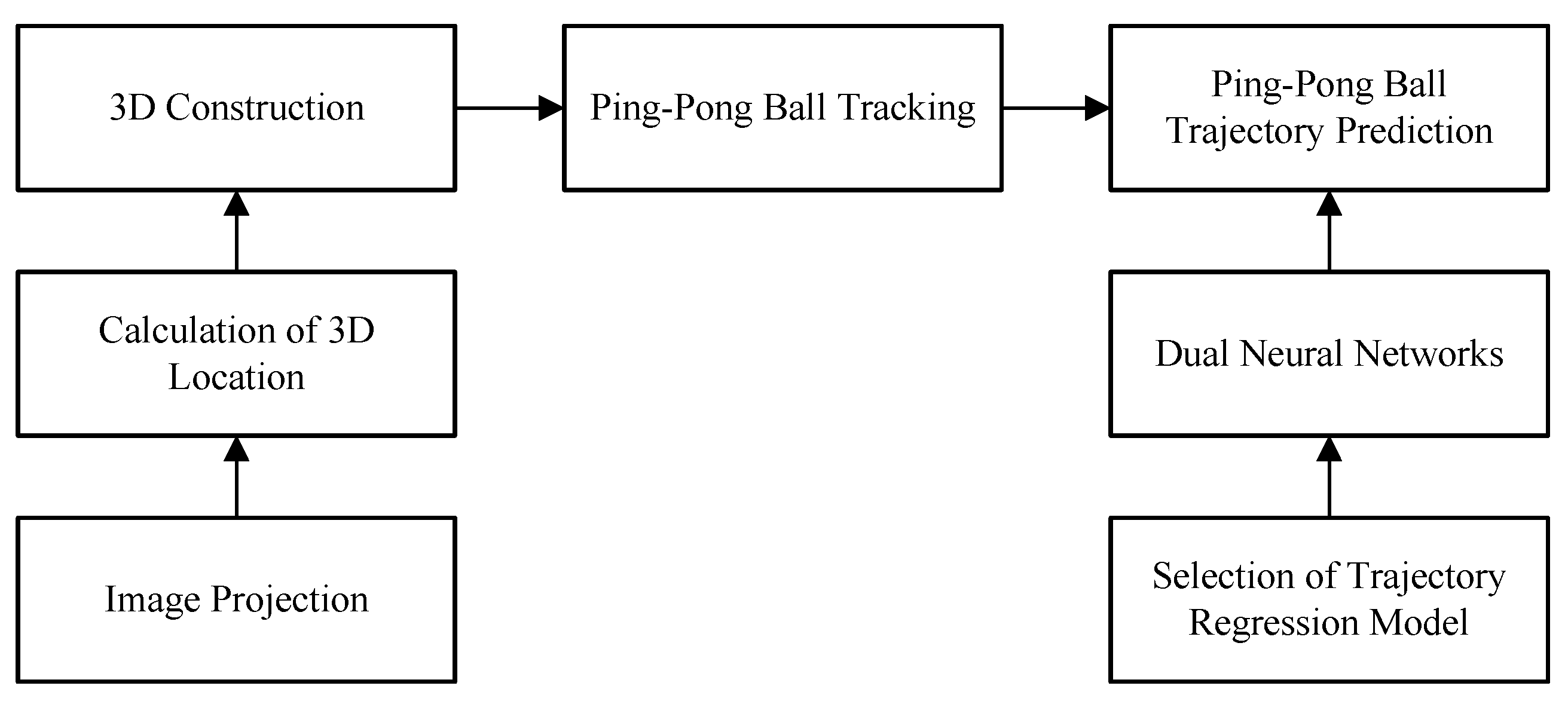
2. 3D Reconstruction Framework
2.1. Hardware Setup
2.2. 3D Reconstruction
2.3. Ping-Pong Ball Tracking
2.3.1. Image Projection
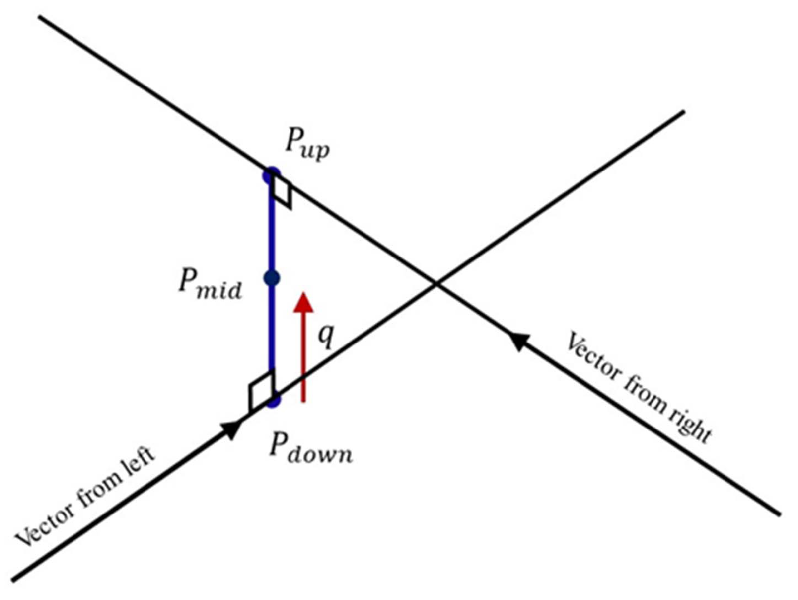
2.3.2. Calculation of 3D Location
2.4. Estimation Error Analysis
3. Ping-Pong Ball Trajectory Prediction
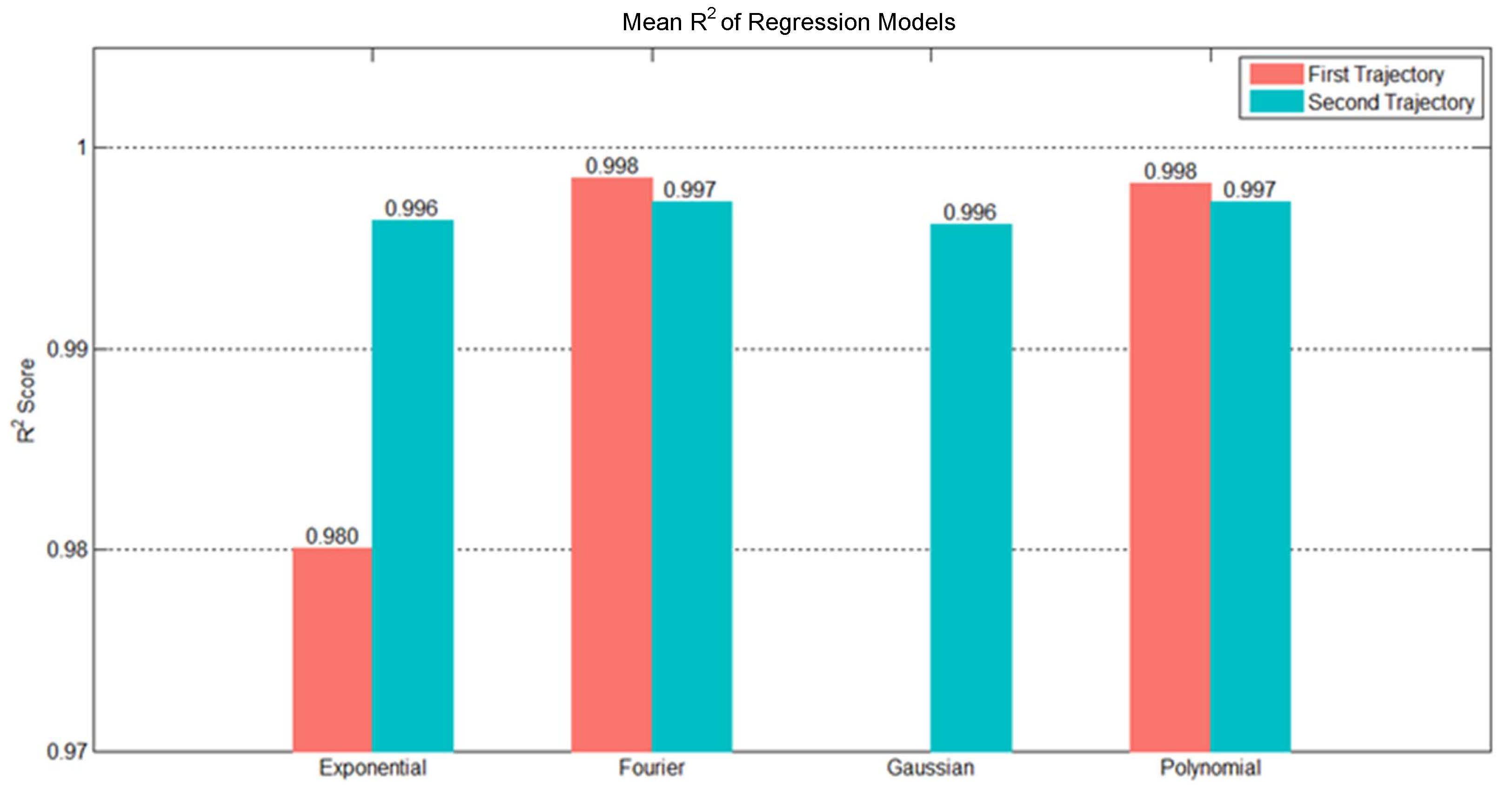
3.1. Selection of Trajectory Regression Model
3.2. Theoretical Verification of Trajectory and Polynomial Coefficients
3.3. Comparison of Artificial Neural Network and Polynomial Curve Fitting Predictions
3.4. Two ANNs in Trajectory Prediction
4. Experimental Results
4.1. Dual-Network vs. Single-Network Approach
4.2. Physical Model Testing
- Using the 330 trajectories, we obtained the mean velocities before and after collision and then the mean collision coefficient. Based on the formula for the coefficient of restitution in Equation (24), we concluded that the mean coefficient was 0.9203.
- The Y and Z positions of the testing trajectories at x = 400 mm (the striking point), i.e., and , were used to calculate the errors in the final prediction results by selecting 100 random trajectories.
- The data from the ten anterior positions of the testing trajectories were obtained, and then the initial velocities in the X, Y, and Z directions, i.e., , , and , using polynomial regression.
- The downward accelerate was defined with air resistance taken into account as shown in Equation (25), where g denotes gravitational acceleration and equals 9.81 m/s2; m is the weight of the ping pong ball, which is approximately 2.7 × 10⁻³ kg; is the resistance coefficient and equals 0.5; denotes air fluid density, which is 1.29 kg/m3; and A is the cross-sectional area of the ball, which is roughly 1.3 × 10⁻³ m2. The mathematical formula indicates that the velocity and acceleration of the object change with time. Here, we set sampling time to be 0.005 s.
- When the ball reached the table (Z direction), we used the mean collision coefficient obtained in the first step to calculate the velocity of the ball after landing, as shown in Equation (29). Once the velocity was calculated, we could continue to calculate the position of the ball in the Z direction.
- Not considering the influences of friction between the ball and the table surface and the self-rotation of the ball, we could calculate the displacement of the ball in the X direction at each sampling time using Equations (30) and (31). The velocity and acceleration of the ball in this direction also changed with time, all the way to the striking point (x = 400 mm). The timing of the striking point, , was then recorded.
- Finally, we used the initial velocity in the Y direction, , air resistance acceleration, in Equation (32), and timing of striking point, , to derive the striking point in the Y direction. Using the predicted Y and Z positions of the striking point, and , and the actual striking point, and (Step 2), we then calculated the error using Equation (33).
4.3. Removal of Time Data
4.4. Striking Point Errors
4.5. Experiment Discussion
5. Conclusions
Author Contributions
Funding
Conflicts of Interest
References
- Shi, Q.; Li, C.; Wang, C.; Luo, H.; Huang, Q.; Fukuda, T. Design and implementation of an omnidirectional vision system for robot perception. Mechatronics 2017, 41, 58–66. [Google Scholar] [CrossRef]
- Koç, O.; Maeda, G.; Peters, J. Online optimal trajectory generation for robot table tennis. Robot. Auton. Syst. 2018, 105, 121–137. [Google Scholar] [CrossRef]
- Zhang, Y.H.; Wei, W.; Yu, D.; Zhong, C.W. A tracking and predicting scheme for ping pong robot. J. Zhejiang Univ. Sci. C 2011, 12, 110–115. [Google Scholar] [CrossRef]
- Li, H.; Wu, H.; Lou, L.; Kühnlenz, K.; Ravn, O. Ping-pong robotics with high-speed vision system. In Proceedings of the 2012 12th International Conference on Control Automation Robotics & Vision (ICARCV), Guangzhou, China, 5–7 December 2012; pp. 106–111. [Google Scholar]
- Liu, J.; Fang, Z.; Zhang, K.; Tan, M. Improved high-speed vision system for table tennis robot. In Proceedings of the 2014 IEEE International Conference on Mechatronics and Automation, Tianjin, China, 3–6 August 2014; pp. 652–657. [Google Scholar]
- Chen, X.; Huang, Q.; Zhang, W.; Yu, Z.; Li, R.; Lv, P. Ping-pong trajectory perception and prediction by a PC based High speed four-camera vision system. In Proceedings of the 2011 9th World Congress on Intelligent Control and Automation, Taipei, Taiwan, 21–25 June 2011; pp. 1087–1092. [Google Scholar]
- Yang, P.; Xu, D.; Zhang, Z.; Chen, G.; Tan, M. A vision system with multiple cameras designed for humanoid robots to play table tennis. In Proceedings of the 2011 IEEE International Conference on Automation Science and Engineering, Trieste, Italy, 24–27 August 2011; pp. 737–742. [Google Scholar]
- Liu, Y.; Liu, L. Accurate real-time ball trajectory estimation with onboard stereo camera system for humanoid ping-pong robot. Robot. Auton. Syst. 2018, 101, 34–44. [Google Scholar] [CrossRef]
- Lampert, C.H.; Peters, J. Real-time detection of colored objects in multiple camera streams with off-the-shelf hardware components. J. Real-Time Image Process. 2012, 7, 31–41. [Google Scholar] [CrossRef]
- Schauwecker, K. Real-Time Stereo Vision on FPGAs with SceneScan. In Forum Bildverarbeitung 2018; KIT Scientific Publishing: Deutschland, Germany, 2018; p. 339. [Google Scholar]
- Zhang, Y.; Zhao, Y.; Xiong, R.; Wang, Y.; Wang, J.; Chu, J. Spin observation and trajectory prediction of a ping-pong ball. In Proceedings of the 2014 IEEE International Conference on Robotics and Automation (ICRA), Hong Kong, China, 31 May–7 June 2014; pp. 4108–4114. [Google Scholar]
- Zhao, Y.; Zhang, Y.; Xiong, R.; Wang, J. Optimal state estimation of spinning ping-pong ball using continuous motion model. IEEE Trans. Instrum. Meas. 2015, 64, 2208–2216. [Google Scholar] [CrossRef]
- Zhang, Z.; Xu, D.; Tan, M. Visual measurement and prediction of ball trajectory for table tennis robot. IEEE Trans. Instrum. Meas. 2010, 59, 3195–3205. [Google Scholar] [CrossRef]
- Wang, P.; Zhang, Q.; Jin, Y.; Ru, F. Studies and simulations on the flight trajectories of spinning table tennis ball via high-speed camera vision tracking system. Proc. Inst. Mech. Eng. Part P J. Sports Eng. Technol. 2019, 233, 210–226. [Google Scholar] [CrossRef]
- Huang, Y.; Xu, D.; Tan, M.; Su, H. Trajectory prediction of spinning ball for ping-pong player robot. In Proceedings of the 2011 IEEE/RSJ International Conference on Intelligent Robots and Systems, San Francisco, CA, USA, 25–30 September 2011; pp. 3434–3439. [Google Scholar]
- Zhao, Y.; Xiong, R.; Zhang, Y. Rebound modeling of spinning ping-pong ball based on multiple visual measurements. IEEE Trans. Instrum. Meas. 2016, 65, 1836–1846. [Google Scholar] [CrossRef]
- Su, H.; Fang, Z.; Xu, D.; Tan, M. Trajectory prediction of spinning ball based on fuzzy filtering and local modeling for robotic ping–pong player. IEEE Trans. Instrum. Meas. 2013, 62, 2890–2900. [Google Scholar] [CrossRef]
- Zhang, Y.; Xiong, R.; Zhao, Y.; Wang, J. Real-time spin estimation of ping-pong ball using its natural brand. IEEE Trans. Instrum. Meas. 2015, 64, 2280–2290. [Google Scholar] [CrossRef]
- Wang, Q.; Zhang, K.; Wang, D. The trajectory prediction and analysis of spinning ball for a table tennis robot application. In Proceedings of the 4th Annual IEEE International Conference on Cyber Technology in Automation, Control and Intelligent, Hong Kong, China, 4–7 June 2014; pp. 496–501. [Google Scholar]
- Nakashima, A.; Ogawa, Y.; Kobayashi, Y.; Hayakawa, Y. Modeling of rebound phenomenon of a rigid ball with friction and elastic effects. In Proceedings of the 2010 American Control Conference, Baltimore, MD, USA, 30 June–2 July 2010; pp. 1410–1415. [Google Scholar]
- Bao, H.; Chen, X.; Wang, Z.T.; Pan, M.; Meng, F. Bouncing model for the table tennis trajectory prediction and the strategy of hitting the ball. In Proceedings of the 2012 IEEE International Conference on Mechatronics and Automation, Chengdu, China, 5–8 August 2012; pp. 2002–2006. [Google Scholar]
- Matsushima, M.; Hashimoto, T.; Takeuchi, M.; Miyazaki, F. A learning approach to robotic table tennis. IEEE Trans. Robot. 2005, 21, 767–771. [Google Scholar] [CrossRef]
- Miyazaki, F.; Matsushima, M.; Takeuchi, M. Learning to dynamically manipulate: A table tennis robot controls a ball and rallies with a human being. In Advances in Robot Control; Springer: Berlin/Heidelberg, Germany, 2006; pp. 317–341. [Google Scholar]
- Zhao, Y.; Xiong, R.; Zhang, Y. Model based motion state estimation and trajectory prediction of spinning ball for ping-pong robots using expectation-maximization algorithm. J. Intell. Robot. Syst. 2017, 87, 407–423. [Google Scholar] [CrossRef]
- Deng, Z.; Cheng, X.; Ikenaga, T. Ball-like observation model and multi-peak distribution estimation based particle filter for 3D Ping-pong ball tracking. In Proceedings of the 2017 Fifteenth IAPR International Conference on Machine Vision Applications (MVA), Nagoya, Japan, 8–12 May 2017; pp. 390–393. [Google Scholar]
- Payeur, P.; Le-Huy, H.; Gosselin, C.M. Trajectory prediction for moving objects using artificial neural networks. IEEE Trans. Ind. Electron. 1995, 42, 147–158. [Google Scholar] [CrossRef]
- Nakashima, A.; Takayanagi, K.; Hayakawa, Y. A learning method for returning ball in robotic table tennis. In Proceedings of the 2014 International Conference on Multisensor Fusion and Information Integration for Intelligent Systems (MFI), Beijing, China, 28–29 September 2014; pp. 1–6. [Google Scholar]
- Zhang, Z. Determining the epipolar geometry and its uncertainty: A review. Int. J. Comput. Vis. 1998, 27, 161–195. [Google Scholar] [CrossRef]
- Biagiotti, L.; Melchiorri, C. Trajectory Planning for Automatic Machines and Robots; Springer Science & Business Media: Berlin/Heidelberg, Germany, 2008. [Google Scholar]


| U Axis | V Axis | Error+ | Error− | |
|---|---|---|---|---|
| Focal Length (pix) | 1043.25281 | 1049.54675 | 2.24798 | 2.12426 |
| Principal Point (pix) | 633.44849 | 561.99736 | 2.89133 | 2.42647 |
| Pixel Error (pix) | 0.26777 | 0.30308 |
| U Axis | V Axis | Error+ | Error− | |
|---|---|---|---|---|
| Focal Length (pix) | 1049.44688 | 1052.73077 | 1.52311 | 1.51341 |
| Principal Point (pix) | 597.44982 | 513.76570 | 2.18344 | 1.66587 |
| Pixel Error (pix) | 0.23623 | 0.26618 |
| X Axis | Y Axis | Z Axis | |
|---|---|---|---|
| Translation vector (mm) | 669.420640 | −371.402272 | 2129.031554 |
| Rotation matrix | −0.821611 | −0.568894 | −0.036249 |
| −0.262626 | 0.434195 | −0.861686 | |
| 0.505947 | −0.698451 | −0.506146 | |
| Pixel Error (pix) | 0.21674 | 0.33150 |
| X Axis | Y Axis | Z Axis | |
|---|---|---|---|
| Translation vector (mm) | −90.227708 | −381.155522 | 2279.359066 |
| Rotation matrix | −0.850091 | 0.526621 | 0.003993 |
| 0.265893 | 0.435734 | −0.859905 | |
| −0.454585 | −0.729936 | −0.510438 | |
| Pixel Error (pix) | 0.15424 | 0.32854 |
| 1st ANN | 2nd ANN | |
|---|---|---|
| Input node number | 40 | 7 |
| Hidden node number | 10 | 20 |
| Output node number | 6 | 7 |
| Activation fun. | Hyperbolic tangent sigmoid | Hyperbolic tangent sigmoid |
| Loss fun. | Mean-square error | Mean-square error |
| Epoch number | 10,000 | 10,000 |
| Optimizer | Levenberg–Marquardt | Levenberg–Marquardt |
| Proposed Dual Networks | Single Network | Physical Model | |
|---|---|---|---|
| Mean (mm) | 39.553 | 42.858 | 57.862 |
© 2020 by the authors. Licensee MDPI, Basel, Switzerland. This article is an open access article distributed under the terms and conditions of the Creative Commons Attribution (CC BY) license (http://creativecommons.org/licenses/by/4.0/).
Share and Cite
Lin, H.-I.; Yu, Z.; Huang, Y.-C. Ball Tracking and Trajectory Prediction for Table-Tennis Robots. Sensors 2020, 20, 333. https://doi.org/10.3390/s20020333
Lin H-I, Yu Z, Huang Y-C. Ball Tracking and Trajectory Prediction for Table-Tennis Robots. Sensors. 2020; 20(2):333. https://doi.org/10.3390/s20020333
Chicago/Turabian StyleLin, Hsien-I, Zhangguo Yu, and Yi-Chen Huang. 2020. "Ball Tracking and Trajectory Prediction for Table-Tennis Robots" Sensors 20, no. 2: 333. https://doi.org/10.3390/s20020333
APA StyleLin, H.-I., Yu, Z., & Huang, Y.-C. (2020). Ball Tracking and Trajectory Prediction for Table-Tennis Robots. Sensors, 20(2), 333. https://doi.org/10.3390/s20020333