1. Introduction
Six-axis force/moment (F/M) sensors enable robots to obtain information about three-dimensional forces (Fx, Fy, and Fz) and moments (Mx, My, and Mz). According to the type of transducer used, six-axis F/M sensors can be classified into the following categories: strain gauge, piezoelectric, capacitor, and optical sensors. Most sophisticated six-axis F/M sensors use strain gauges. In a strain gauge sensor, the elastic body in the sensor transfers the applied load to the bonded strain gauge; the gauge then measures elastic deformation. Simultaneously achieving high sensitivity and decoupled outputs with a low cross-talk error in six-axis F/M sensors is challenging.
Decoupled six-axis F/M sensors proposed by previous studies can be classified into two groups: mechanically decoupled sensors and sensors using decoupling algorithms. In a parallel three-dimensional force sensor proposed in a previous study, mechanical decoupling was implemented to reduce the influence of dimensional coupling and improve sensing accuracy [
1]. However, most existing six-axis F/M sensors lack complete integration. Therefore, instead of using mechanical decoupling methods, researchers have developed various decoupling algorithms using simple and convenient methods, such as linear regression [
2] and the least squares method (LSM) [
3,
4,
5], and advanced methods, including neural networks, the shape-form-motion approach [
6], support vector regression (SVRs) [
7,
8], and least squares support vector machines (LS-SVMs) [
9].
Regarding the development of the structures of F/M sensors, particularly the elastic body, design is critical to ensure optimal sensor performance. Many researchers have designed elastic body structures in the form of E-type membranes [
10], T-shaped bars [
11], Stewart platform [
12], parallel plates [
13], parallel beams [
14], and Maltese crossbeams [
15]. In a previous study, a cross-shaped double-hole structure was improved by considering structural errors resulting from the inaccuracy of the sensor body and by performing signal conditioning for noise reduction [
16]. A previously proposed sensor involving a Maltese cross element with rigid inner and outer flanges can measure specific components of external forces; however, it has low sensitivity to horizontal forces (
Fx and
Fy), which subsequently causes considerable cross coupling [
11].
A study proposed a numerical shape optimization design for a mechanically decoupled six-axis F/M sensor [
17]. Moreover, scholars have proposed optimization methods for validating structural analysis models using conditional numbers, static and dynamic stiffness, and strain gauge sensitivity as sensor design parameters. A study optimized the design of a thin-type four-axis F/M sensor for a robot finger by applying structural optimization techniques in which strain gauges were positioned using a response surface method and a suitable function [
18]. In another study, four identical T-shaped bars were subjected to finite element analysis (FEA) along with design optimization to maximize measurement sensitivity [
11]. Furthermore, studies [
19,
20] have presented the Stewart platform that can achieve a comprehensive index optimization of the structural parameters of a force sensor by using indices atlases and a genetic algorithm. In another study, the performance and structural design of a prestressed six-axis F/M sensor with double layers were validated by considering the optimization objective to obtain optimal structural parameters [
21]. To optimize the design of a multi-axis force sensor (MFS) integrated in a humanoid robot foot structure, a study analyzed the design criteria and strain gauge sensitivity as the objective function for MFS numerical optimization [
22]. However, developing an F/M sensor with high performance requires appropriate design criteria for the sensor’s body structure and a numerical optimization process to evaluate the sensor’s sensing accuracy in terms of cross coupling and measurement error.
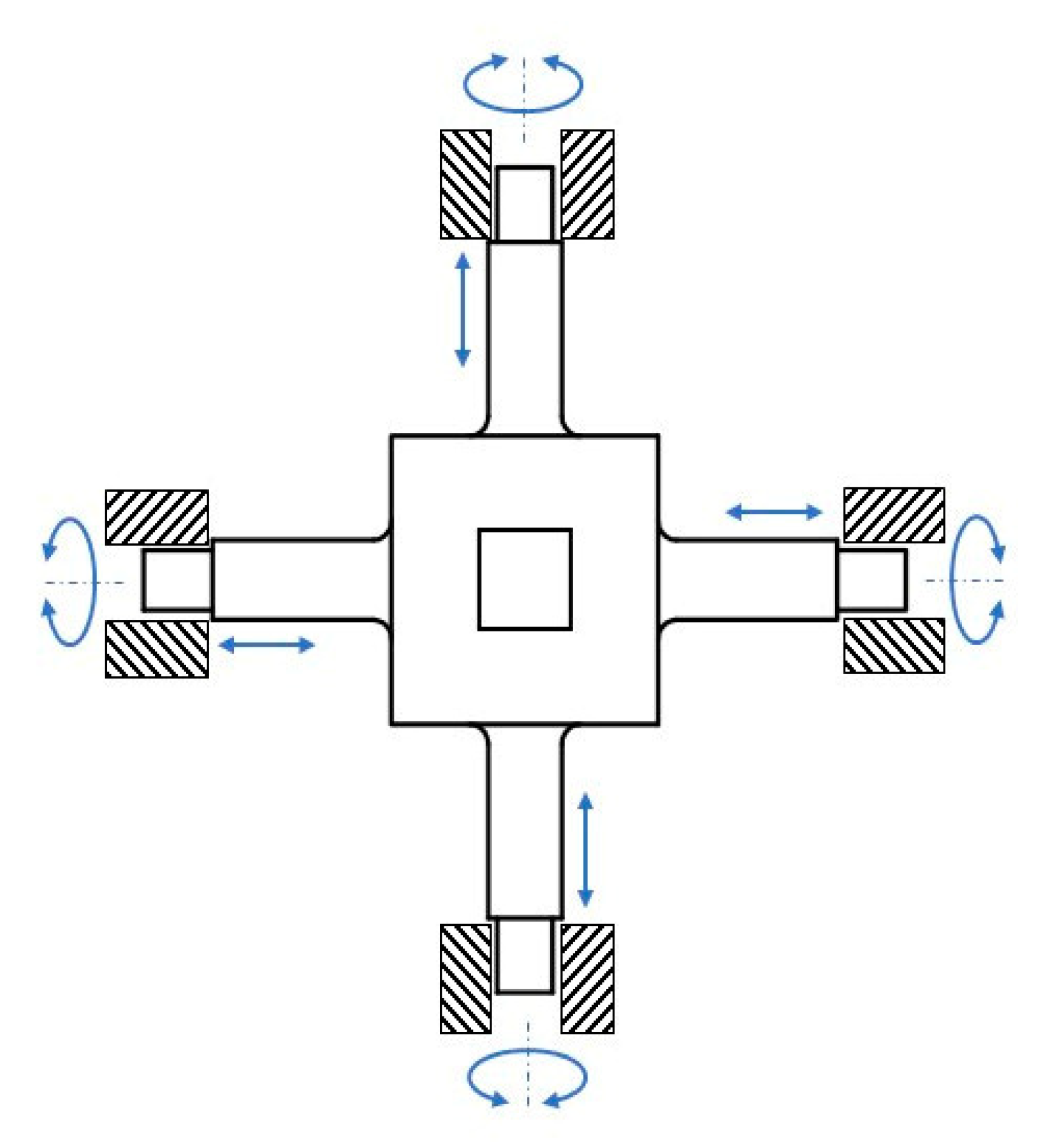
A precise sliding and rotating clearance between the symmetrical grooves and elastic body is necessary to decouple a structure. Otherwise, the contact force between the elastic body and the groove’s sidewall affects the structure. This study presents a novel mechanically decoupled six-axis F/M sensor with a sliding and rotating cross-elastic beam structure afforded by a unique strain gauge configuration [
23]. In addition, this paper describes the theoretical calculation of the deformation, stress, and strain of the proposed six-axis F/M sensor through analytical modeling. The decoupling relationship between the sliding and rotating mechanisms is also analyzed herein through cross-talk error performance. On the basis of a mechanical and analytical model of the sensor and parameters affecting the strain values for the six-axis F/M sensor, stress and strain distributions are described herein [
24].
The rest of this paper is organized as follows.
Section 2 presents the decoupled structural design and strain gauge configuration of the proposed six-axis F/M sensor.
Section 3 describes the design requirements and analysis of the sliding and rotating structure of the F/M sensor.
Section 4 presents the results and discussion, including a comparison of numerical and analytical solutions for the optimized design structure of the F/M sensor, the results of friction analysis, and the results of experimental validation. Finally,
Section 5 provides the conclusions.
3. Structural Analytic Solution
Plastic deformation occurs when the F/M-induced stress on a flexure exceeds the yield strength of the flexure. The structural part of the elastic body is crucial for the F/M sensor design. In the F/M sensor structure design proposed in this paper, the strains of the elastic beam structure are fully analyzed using Timoshenko beam theory [
27]. In this design, symmetry with respect to loads in the
x and
z directions is determined through a bending analysis for a single cantilever module. This section describes the design requirements and the analysis of the sliding and rotating structure of the F/M sensor.
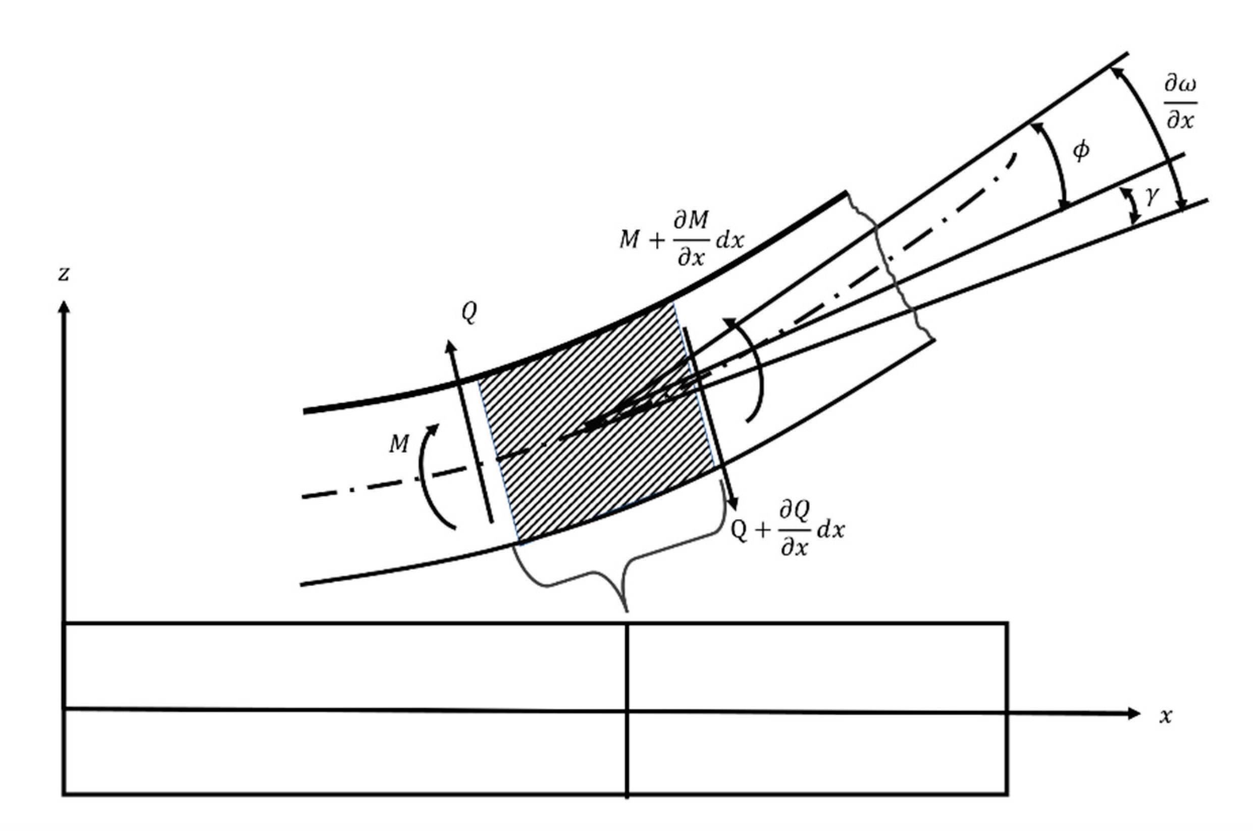
In Timoshenko beam theory, illustrated by
Figure 5, the bending moment is denoted by
M and the shearing force is denoted by
Q [
27]. Let
ϕ be the angle caused by bending and
γ be the angle caused by shear. Beam deformation characteristics are described by two unknown parameters: the translational displacement (
ω) and angular displacement (
φ) of any cross section in terms of
x. The coordinate value of any point on the beam can be expressed as follows:
The F/M equilibrium equations for the infinitesimal element of the beam are based on Equation (2). The following ordinary differential equations can be obtained after linking Equation (2) with the infinitesimal element of the beam:
where
EI is flexural rigidity,
κ is a constant depending on the shape of the cross section of the beam, A is the cross-sectional area, and
G is the modulus of rigidity. Therefore,
and
is the cross-sectional area of the elastic beam.
The two basic formulas in Timoshenko beam theory are presented in Equations (2) and (3) and can be used to calculate an analytical solution of
ω(
x) and
φ(
x) if sufficient boundary conditions are provided. The strain value (
ε) of any point on a beam can be calculated using Equation (4) after the analytical solution of the angular displacement
φ(
x) is obtained:
where
z is any point along a beam’s
z coordinate; it also indicates the distance between the point and the neural plane.
The following sections present the proposed mechanical model for elastic beams when pure forces or pure moments are applied to the elastic body. The sections also present the effects of these forces or moments on the strain distributions of the elastic body.
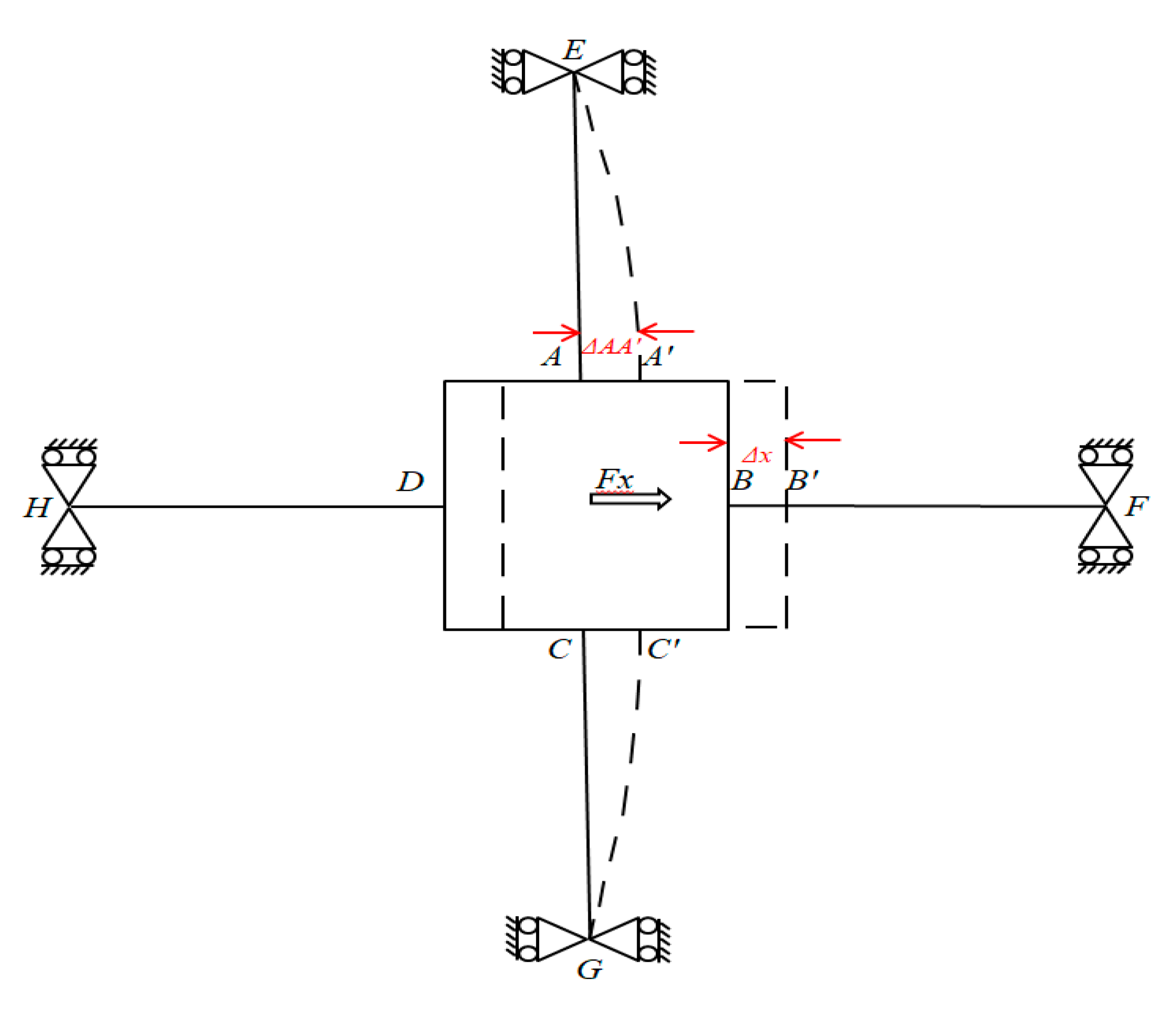
3.1. Under Applied Force Fx or Fy
When a pure force
Fx is applied to the F/M sensor (
Figure 6), the axial forces are transmitted through elastic beams
DH and
BF to produce a sliding motion in the elastic body of the non-contact force sensor (i.e., no bending deformation occurs). Concurrently, bending deformation occurs in beams
AE and
CG.
A′,
B′, and
C′ represent the displaced positions of
A,
B, and
C, respectively. Δ
x,
, or
ω represents the displacement of the rectangular box (i.e., the displacement node of
A in elastic beam
AE). The bending of beam
AE is the same as that of beam
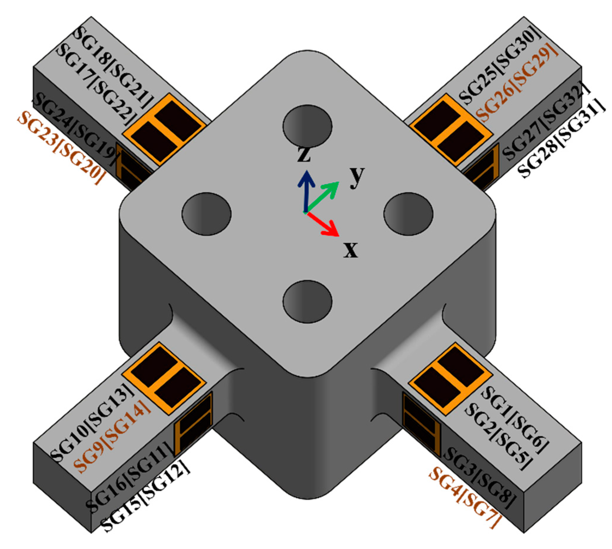
CG. The bending stress levels observed on the strain gauges of the two horizontal beams are equal. We can assume that the output of the strain gauges (SG
15, SG
28 and SG
12, SG
31) regarding the bending stress levels of the two elastic beams (
AE and
CG) are equal.
The force equilibrium equation of the rectangular box can be derived as expressed in Equation (5), where
is the shear force on cross-elastic beam
AE. can be obtained using a combination of Equation (2) and boundary conditions of Equation (3) observed from beam
AE in
Figure 6 and expressed as follows:
By substituting Equation (5) into Equation (6) and then substituting the result into Equation (3) and then Equation (4), we obtain
as a function of
Fx as follows:
3.2. Under Applied Force Fz
When a pure force
is applied to the F/M sensor (
Figure 7), bending deformation occurs on all elastic beams (
AE,
BF,
CG, and
DH). The outputs of the strain gauges (SG
1, SG
18 and SG
6, SG
21) regarding the bending stress levels for the four elastic beams are equal. The geometrical characteristics of the deformation of the beams are illustrated in the free body diagram in
Figure 7. All elastic beams have fixed boundary conditions at nodes
E,
F,
G and
H, corresponding to simply supported beams. Δ
z,
or
ω represents the displacement of the rectangular box (i.e., the displacement node of
A in elastic beam
AE).
The force equilibrium equations of the elastic body are expressed as follows, where
represents the shear force in elastic beam
AE.
As displayed in
Figure 7,
represents the vertical distance between node
and node E.
can be derived using Equation (2) and the boundary conditions in Equation (3) obtained from elastic beam
AE in
Figure 7, and it can be expressed as follows:
where
represents the strain at any point on the elastic beam under
Fz loading, which is derived by substituting Equation (8) into Equation (9), then into Equation (3), and finally into Equation (4):
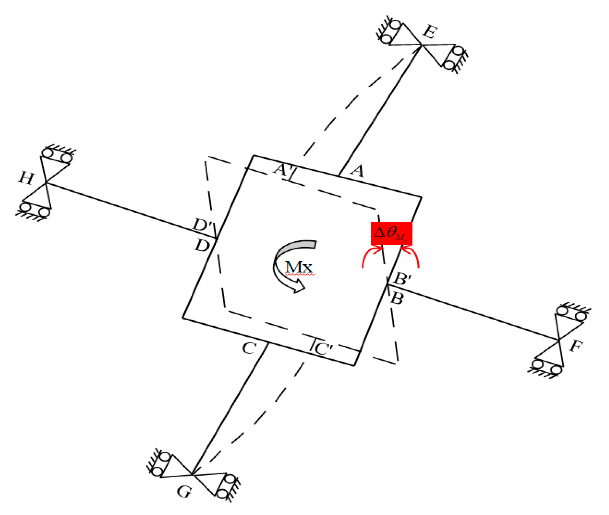
3.3. Under Applied Moment Mx or My
When a pure moment
is applied to the F/M sensor, elastic beams
DH and
BF produce a pure rotating motion following the elastic body of the non-contact force sensor (i.e., no bending deformation is produced). Concurrently, bending deformation occurs in elastic beams
AE and
CG. The bending of elastic beam
AE is similar to that of elastic beam
CG.
Figure 8 presents the deformation of the elastic body under the applied moment
, where
or
φ represents the angle of rotation of the rectangular box with respect to x-axis in global coordinates. The outputs of the strain gauges (SG
13, SG
25, SG
10, and SG
30) regarding the bending stress levels of the two elastic beams (
AE and
CG) are equal.
The F/M equilibrium equation of the elastic body is expressed as follows:
where
is the bending moment on the upper surface of beam
AE, and
The geometric characteristics of the deformed elastic body under the applied
Mx can be calculated using Equation (2) and the boundary conditions in Equation (3) obtained from the deformed characteristics of beam
AE:
where
d represents the distance from the center to node
A on the rectangular box.
The strain value under
Mx loading at any point on the elastic beam, represented by
, can be derived by substituting Equation (11) into Equation (12) and then into Equation (3), followed by substituting the results into Equation (4):
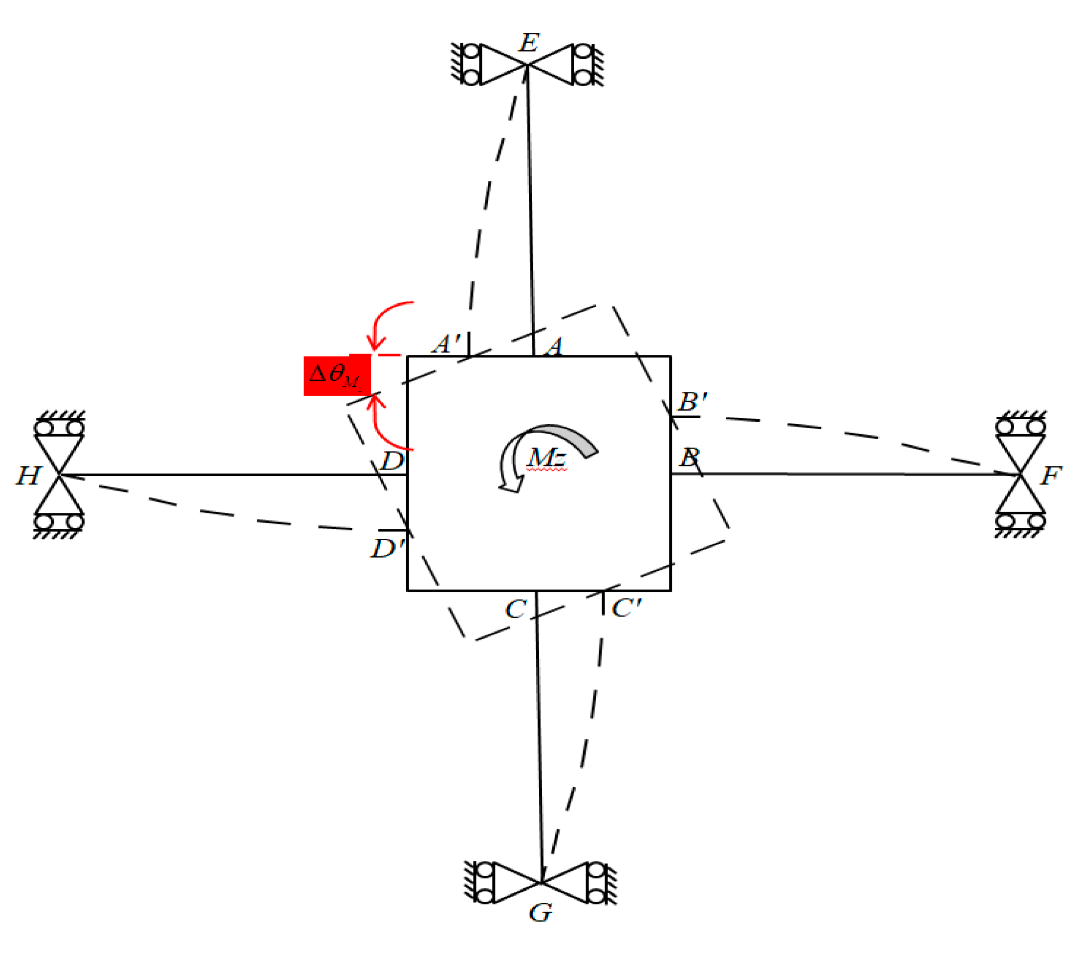
3.4. Under Applied Moment Mz
When a pure moment
is applied to the F/M sensor, bending deformation occurs on all elastic beams (
AE,
BF,
CG, and
DH). The outputs of the strain gauges (SG
16, SG
32 and SG
11, SG
27) regarding the bending stress levels corresponding to the four elastic beams are equal. The geometric characteristics of deformation are illustrated in the free body diagram in
Figure 9. All elastic beams have fixed boundary conditions at nodes
E,
F,
G, and
H, corresponding to simply supported beams.
or
φ represents the angle of rotation of the rectangular box with respect to the z-axis in global coordinates under the applied moment
.
The F/M equilibrium equation of the square convex under
can be expressed as follows:
where
and
are the shear force and bending moment of the upper surface of
AE, respectively, and
.
The angle of rotation
derived using Equation (2) and the boundary conditions in Equation (3) obtained from beam
AE can be expressed as follows:
Similarly, substituting Equation (14) into Equation (15), then into Equation (3), and finally into Equation (4) can yield the strain value
under
Mz loading:
4. Results and Discussion
During the design of a six-axis F/M sensor, several design factors should be considered, including the elastic body’s specific force geometry, sensing element, material, sensing bridge design, stress-strain limits, measuring force limits, and size limitations. The strain can be determined using Timoshenko beam theory and validated using FEA simulation.
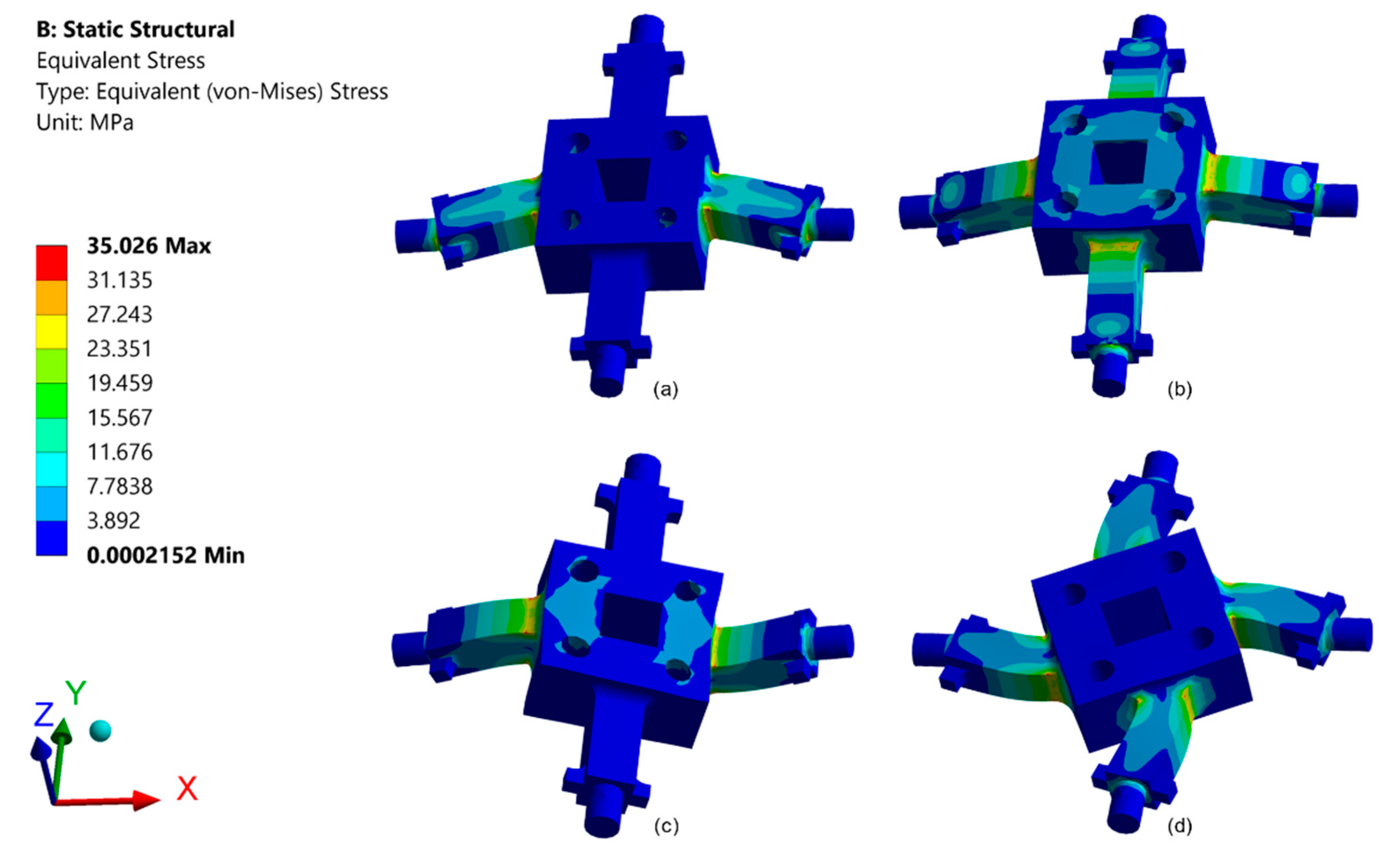
4.1. Numerical Simulations
As presented in
Figure 10, this study simulated an FEA model to analyze the design parameters for the sensor structure in order to confirm the strains calculated using the derived equations under
Fx and
Fz and
Mx and
Mz. The ANSYS program was used for the numerical solutions. The strain gauges for the
Fx,
Fy,
Fz,
Mx,
My, and
Mz components were attached 3 mm from the edge of the rectangular box along the direction of the elastic beam’s length.
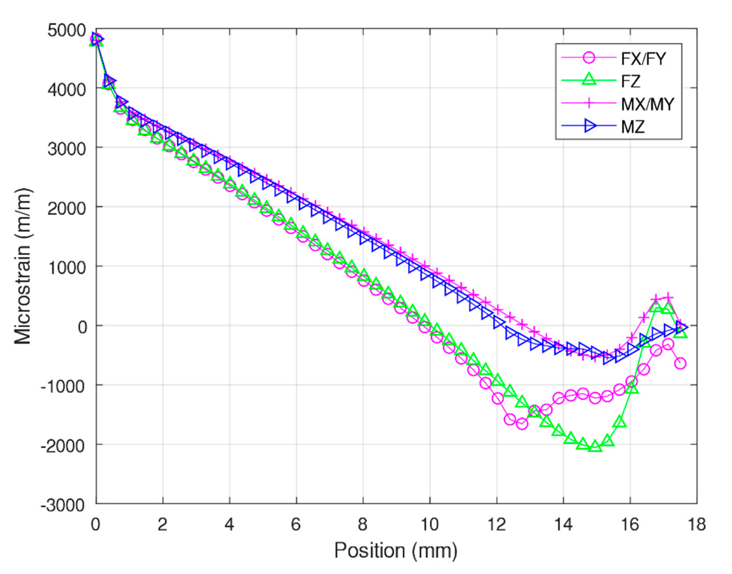
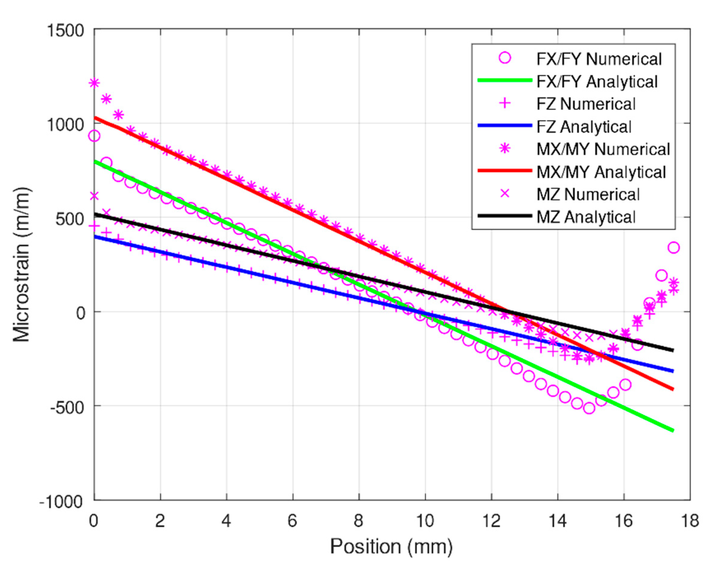
4.2. Comparison of Numerical Solution with Analytical Solution
In the analytical experiment, the Timoshenko equation was modified because it was designed for fixed or pin-type supports only. Because the edges were designed to slide at the end of the elastic beams in this study, constants must be added to the Timoshenko equation. These constants were added according to
Figure 4. These constants were derived at points where the strain was equal to zero and started to turn negative. Consequently, the Timoshenko equation was adjusted and is expressed as follows:
The analysis was conducted using the desired forces:
Fx/
Fy = 400 N,
Fz = 800 N,
Mx/
My = 30 Nm, and
Mz = 30 Nm. The simulation was performed using ANSYS, and normal strain data were obtained at the center of the surface of the elastic beams, as illustrated in
Figure 11. An analytical solution was also obtained using the modified Timoshenko equation and is presented alongside the results of the numerical analysis in
Figure 11. These results demonstrate that the results of the modified Timoshenko equation are similar to the numerical results. However, the final tail of the graph for the numerical results is shown to indicate non-linear strains, whereas the graph for the Timoshenko equation results shows only a straight line. These results agree with those of studies that have compared Timoshenko results with numerical results [
22,
27].
This study focused on the strain gauge placement position on rectangular elastic beams at a distance of 3 mm from the center box.
Table 2 presents a comparison of the numerical simulation results and the analytical solutions. When
My = 30 Nm, the largest error was 2.51%. The corresponding error in [
25] was 7.7%, which implies that our modified Timoshenko equation is superior.
This structure is then tested to quantify the cross-talk errors generated by Equation (18) as shown in
Table 3. This equation is well known among researchers, to name a few studies undertaken by [
14,
17,
28] which using this equation is used to make cross-talk error. The largest cross-talk error generated in this study was 0.35%. In an ANSYS-based study conducted previously that involved the same configuration as that used in the present study [
23], a cross-talk error of 11% was obtained. Therefore, our proposed sensor with a sliding structure is superior to sensors without sliding structures. Another study [
29] proposed a sensor with sliding structures and double-type elastic cross beams; for this sensor, the maximum error generated was 0.89%. However, the difference between this sensor and that proposed in the present study is the strain gauge configuration. The strain gauge configuration in the sensor proposed in the present study is considerably more suitable for sliding mechanisms.
Sij is the measured strain, with i = 1, …, 6 representing the measurement provided by the strain gauge bridge and j = 1, …, 6 representing the specified load on the force sensor. For example, S11 represents the reading provided by strain gauge bridge Fx (SG FX) when Fx is applied to the force sensor (Equation (1)). When i ≠ j, a cross-talk error may occur on the force sensor. For example, S12 indicates the reading provided by SG Fx when Fy is applied.
4.3. Optimization
The Timoshenko equation could result in relatively low errors and could facilitate the execution of optimization processes. Sensor optimization is typically performed to obtain a more acceptable range of measurements and accurate and durable sensor products. The objective of optimization is to attain specific strain levels on each axis to maximize sensitivity. In this study, optimization was performed using sequential quadratic programming, a widely employed method [
24,
30,
31]. To protect the strain gauge under an elastic state, the specific strains for each axis were set as follows:
SFX =
SFY =
SFZ = 200,
SMX =
SMY = 600, and
SMZ = 300. The loading levels applied in each direction were as follows:
Fx =
Fy = 400 N,
Fz = 800 N,
Mx =
My =
Mz = 30 Nm. The design variable [
b,
h] was determined such that
(attain factor) was minimized; this could be achieved using the following equation:
The design optimization process resulted in the elastic beam width (
b) and thickness (
h) listed in
Table 4.
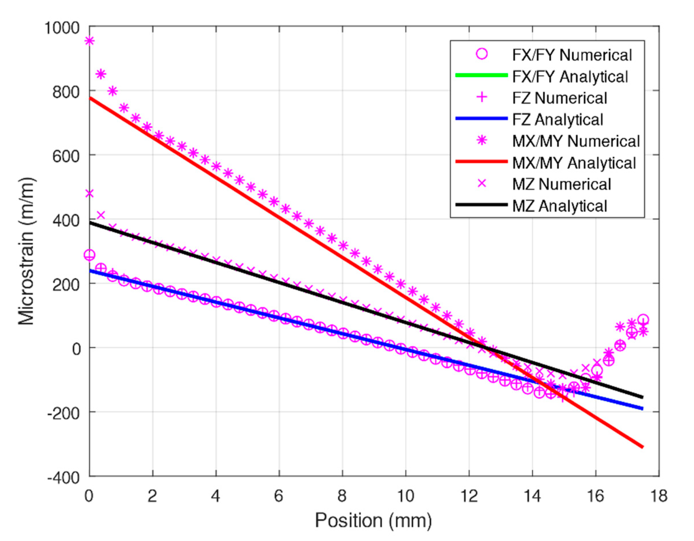
Because this study yielded new optimized structural parameters, additional simulations were required. One of the simulations was conducted using the modified Timoshenko equation, and the other was conducted through a numerical analysis. As illustrated in
Figure 12, the results obtained using the modified Timoshenko equation were similar to the numerical analysis results. Moreover, the results for
Fx/
Fy and
Fz were similar; therefore, the plot for
Fz cannot be observed in the figure. According to the optimized structural dimensions, strain analysis was performed on the specified strain gauge configuration throigh both numerical simulation and numerical analysis. As presented in
Table 5, the errors generated for
Fx/
Fy and
Fz were nearly negligible, but those for
Mx/
My and
Mz were substantial. However, compared with the 7.7% deviation reported by a previous study [
26], the result of the present study is superior.
A cross-talk error analysis was performed for the sensor with the optimized structure. As revealed in
Table 6, the largest error was observed for
Fy (0.51%), which is relatively high compared with the results of related studies. However, the error is controllable and this is more favorable than that reported by a previous study [
29] that utilized a sliding framework and achieved a maximum error of 0.89%.
4.4. Friction
The simulation and analysis results presented in the preceding sections are suitable for structures in which antifriction bearings are used between the elastic body and the upper and lower rims (housing part). When a dry-sleeve bearing is used, which is small, low maintenance, and without a lubricant, it may cause minimum friction, with the corresponding friction coefficients being approximately 0.01–0.20. Therefore, some inaccuracies may be produced.
Table 7 shows the results of a friction analysis conducted on a sleeve bearing with a friction coefficient of 0.20. The design of this analysis was based on the initial design presented in
Table 1. Values presented in boldface type in
Table 7 represent errors pertaining to the non-frictional strain analysis. The highest error achieved was 0.58% under
Fz, and the friction increased the cross-talk error. The highest cross-talk error observed for the
Mx sensor under
Fx was −0.53% which is still less than the previous study [
23].
4.5. Experimental Validation
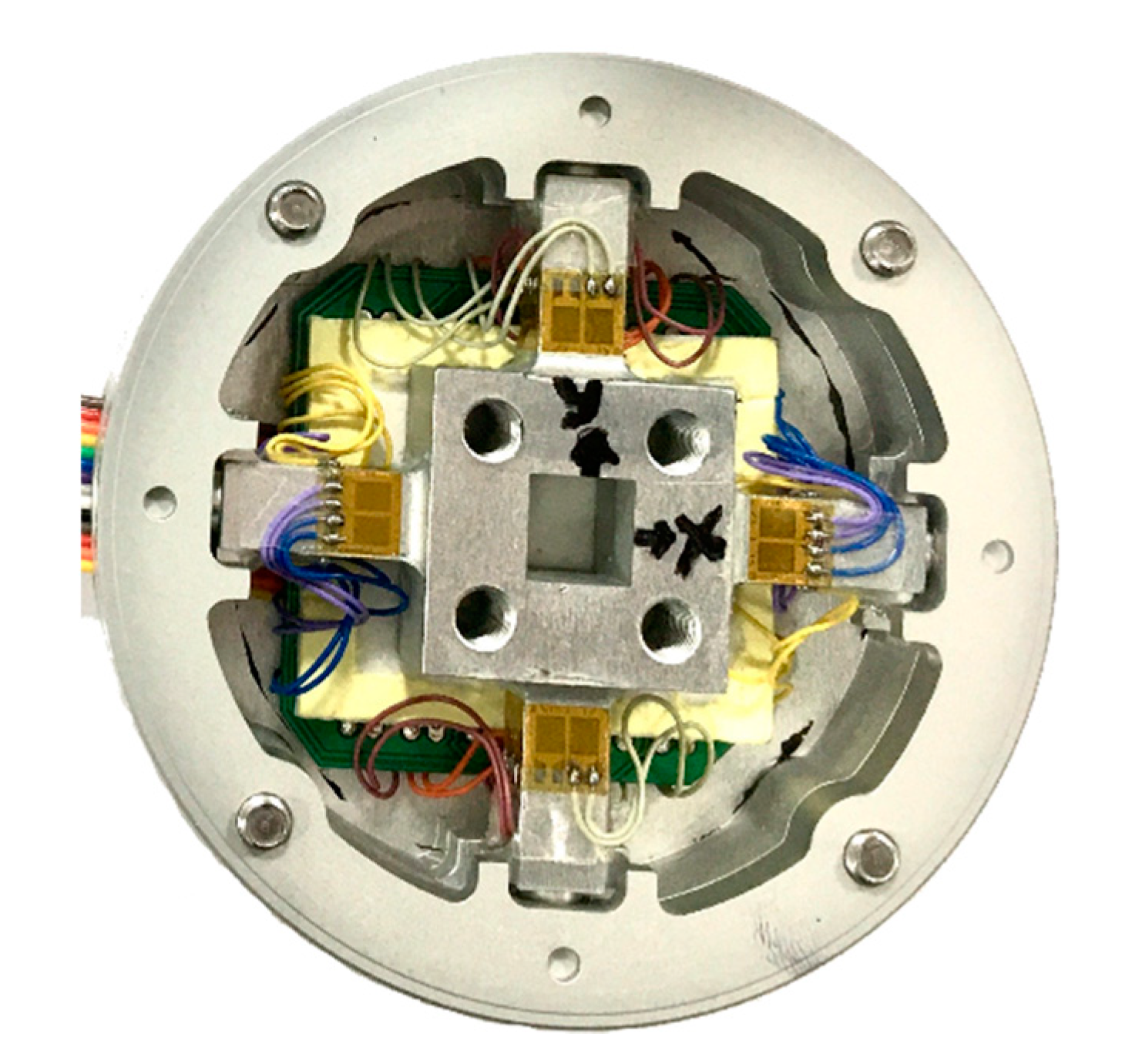
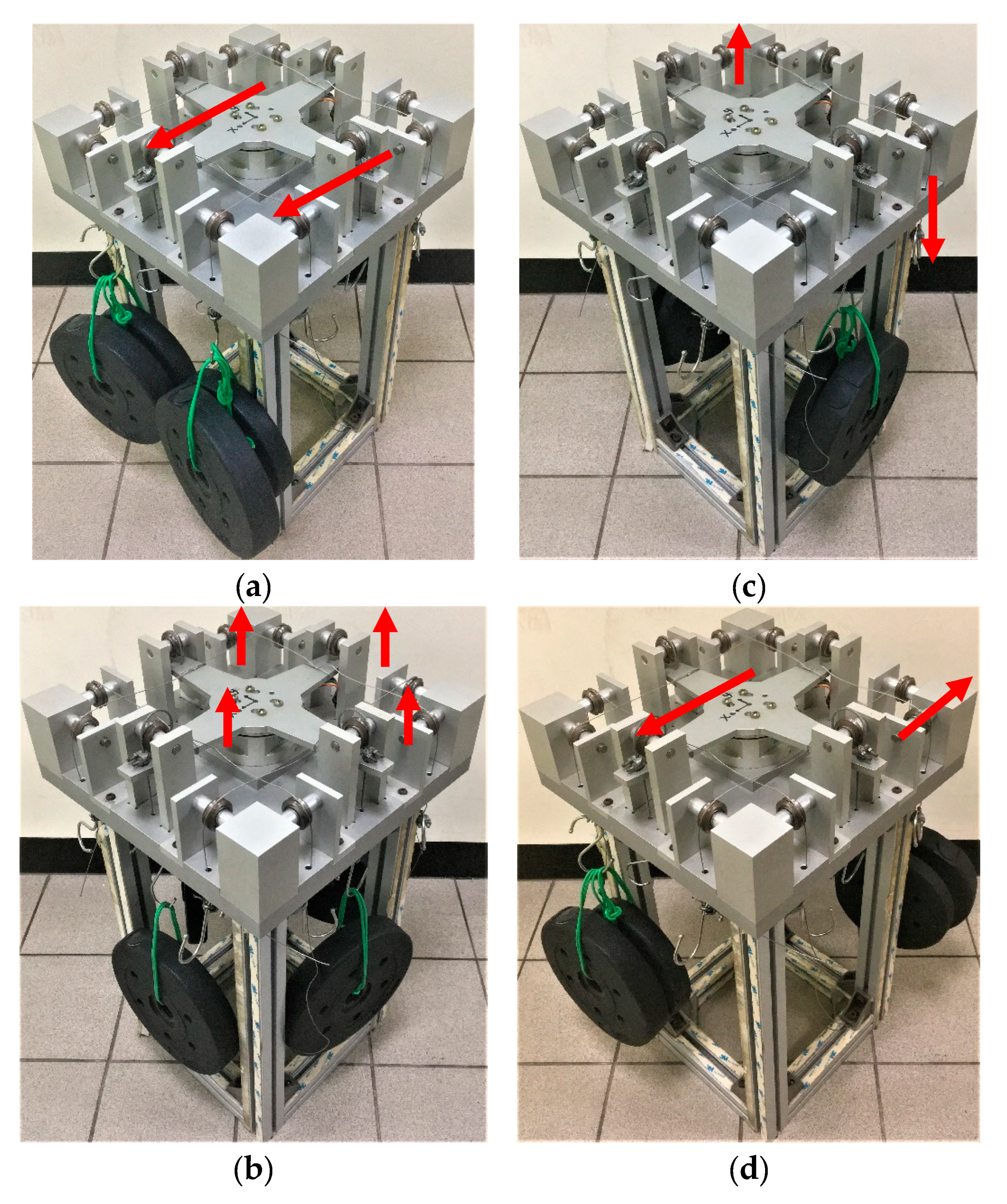
Experimental testing is necessary to obtain a clear evaluation of a novel model. Accordingly, this study conducted an experiment for the proposed sensor. A prototype of the sliding force sensor (
Figure 13) was manufactured on the basis of the initial design presented in
Table 1. A dry-sleeve bearing composed of bronze material was used in the force sensor. The first step in the experiment was to calibrate the sensor (
Figure 14) using the LSM. After the calibration, the sensor was tested to determine its performance.
Table 8 presents the average output error and cross-talk error. The values in boldface type in the table represent the error readings for the applied forces under a specific load. Maximum measurement error was 2.00% and the maximum cross-talk error occurred when
Mz loading on
SFx was 2.63%.
The measurement error obtained in this paper showed some error difference compared to the previous study [
23], which could have been 1.78%, even with the same strain gauge arrangement. But if we equate the cross-talk error, the present study shows a significant improvement from 4.78% to 2.63%. Nonetheless, if we equate it with studies [
28] that use LSM to get calibration matrix, the measurement error they obtain is 6.85% and the crosstalk error is 4.85%. Therefore, the development of the force sensor compared to the manufactured prototypes has been achieved.
Looking at the simulation test, this model is expected to achieve the best performance so far. The real challenge is to make it so that the result would be the same with the simulation. The manufacturing process of the sensor has always faced a structural error of the body and the bonding process effect of the strain gauge leads to a minor error from analysis to experimental testing.


