Real-Time 3D Reconstruction of Thin Surface Based on Laser Line Scanner


Abstract
:1. Introduction
2. Methodology
2.1. Truncated Signed Distance Field (TSDF) Computation from 3D Curves
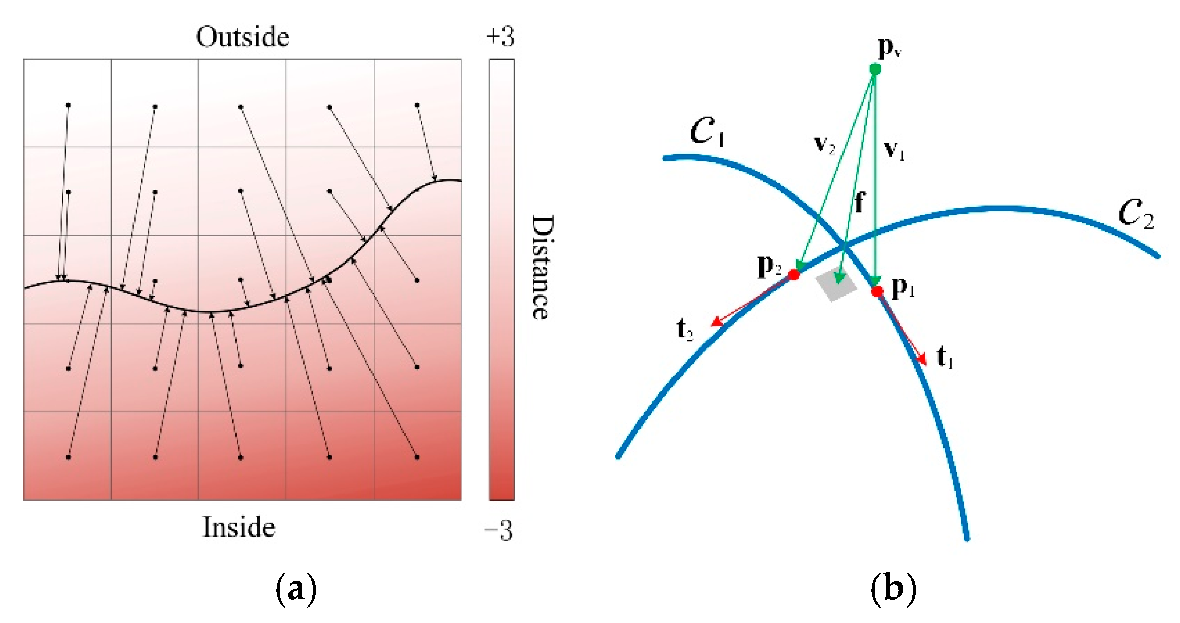
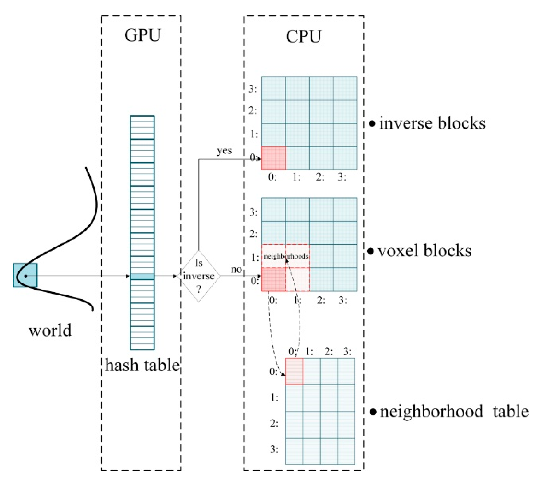
- Voxels Allocation: after receiving a frame of 3D curves data, we compute the pv of all voxels that fall within the fundamental envelopes of the curves and find the corresponding voxel block of pv in the hash table. If no block is found, we allocate a new block for it on the heap;
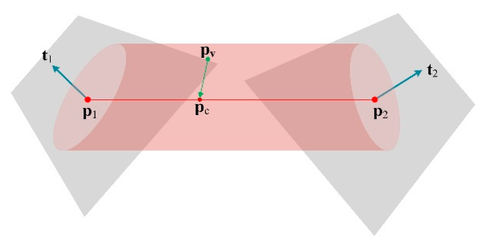
- TSDF Computation: compute the TSDF observations of these voxels (including the closest point pc on the curve and tangent tc on pc);
- Voxels Indexing: use pv to index the address of voxel v in hash table;
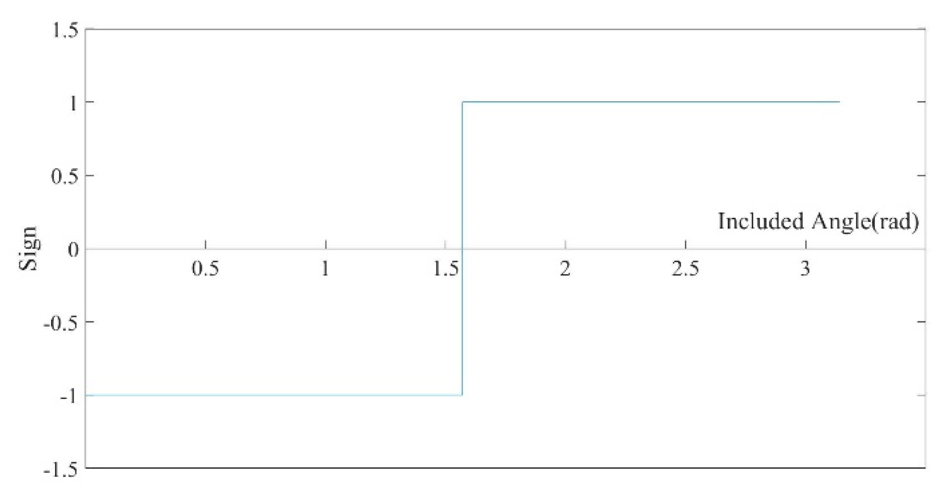
- Voxel Integration: before integrating the new TSDF, it is necessary to determine whether the new one is on the same side as the surface already encoded by v. If so, the new TSDF is integrated to voxel v by Equations (6)–(8) (updating weight ω, matrix C and distance vector ). Conversely, we find the inverse voxel v’ on the other side of the thin surface and update v’. The method of determining which side of the thin surface the current observation belongs to will be elaborated in the next section;
- Normal filtering: the surface normal plays a vital role in the judgment of thin-surface attribution, and also affects the real-time display quality. Therefore, we need to denoise it to make it reliable. Firstly, the surface point pc (Equation (4)) and normal n (through a singular value decomposition (SVD) of matrix C) encoded by voxel v are computed. Then the neighborhood points of v are found in the hash table, and n is recomputed with the surface points and normals of v’s neighbors. The related content of normal filtering will also be described in the next section.
- Weak Topological Regions Repair: although we have distinguished the opposite sides of the observed thin surface when integrating voxels, it is difficult to distinguish them in some areas with complex topology. When the user stops scanning, we adopt a post-processing method to detect and repair the topological errors in these areas automatically.
- Isosurface Extraction: after repairing the topological errors in TSDF, we use the marching cubes algorithm to extract the isosurface and generate a mesh model.
2.2. TSDF for Thin Surface
- One Side Visible: when the line of sight is oriented toward one side of the thin surface, the sensor can only measure the current side and cannot measure the opposite side because the dominant side occludes it.
- Both Sides Visible: when the line of sight is approximately parallel to a thin surface and perpendicular to the edge of a thin surface, the thin surface on the opposite sides near the edge can be observed.
- Perform the approach proposed in [6] to estimate the first normal nf and compute the reliability measure λr of nf;
- For each voxel v in the field, estimate the normal ns based on an anisotropic neighborhood;
- Update the normals by combining the first normal nf with ns under the influence of coefficient λr until either convergence or a maximum number of iterations is reached.
2.3. Repairing Weak Topological Regions
2.3.1. Detecting Weak Topological Regions
- Find the critical points: find all voxels in a neighborhood with v as the center. vi is divided into two sets, one f(vi) > f(v) is defined as positive, and one f(vi) ≤ f(v) is defined as negative. Within each set, adjacent voxels are joined together to obtain several connected groups Γi±, as shown in Figure 9. If the number of connected groups of v is 2, then v is not the critical point. If the number of connection groups of v is 1 or ≥ 2, then v is a critical point;
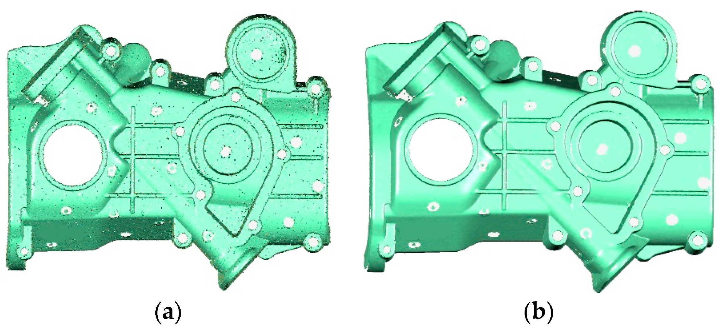
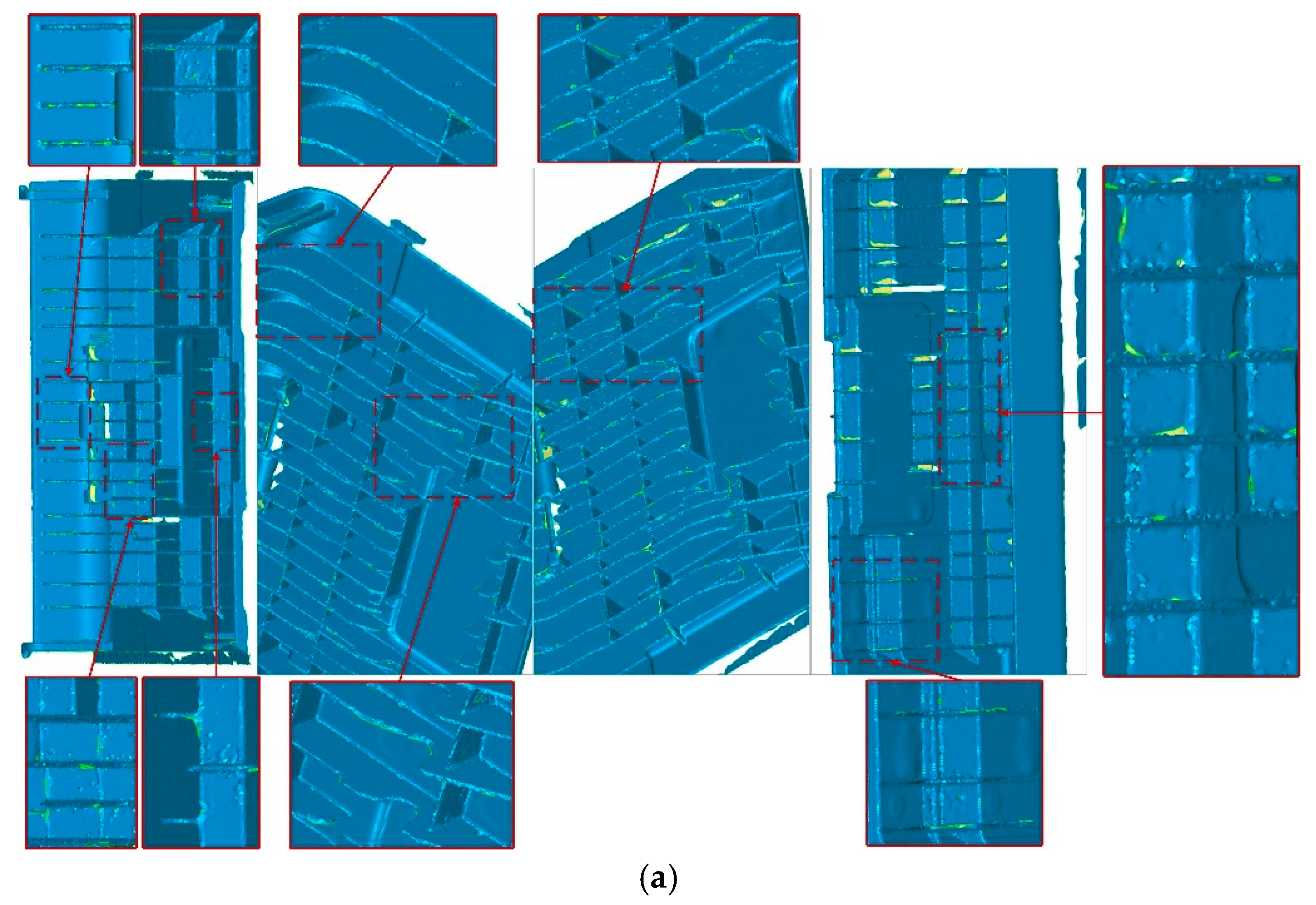
- Generate weak topological regions: take each critical point Pc as a seed point, find connected component Pg (a region of adjacent voxels) of Pc within a specified range (such as two times of the voxel size), and the dot product of the normal less than a certain threshold Tdot. Figure 10 shows weak regions detected by our method. This model has many stiffeners with a thickness of about 1 mm. When the truncation is also set to 1 mm, the surface model is prone to generate topological errors in the location of these stiffeners. The proposed method can detect these weak topological regions (the red areas in the figure), and the method of repairing topology errors will be described in the next section.
2.3.2. Repairing Weak Topological Regions
2.4. Data Structure
| Algorithm 1. Computation of the TSDF from a set of curves. |
| Input: Set of curves ci = {pi,1, …, pi,ni}, i[1,N]; tangent ti,j at each point pi,j, j[1,n]. Output: TSDF: . 1: Initialize matrix C, distance vector and weight ω in all voxels to zero 2: for each curve i[1, N] (number of curves) do 3: for each point j[1, n] (number of points on the curves) do 4: Compute the bounding box of the line segment ; 5: for all voxels pv (the central point of the voxel) in the bounding box do 6: if pv is in the fundamental envelope associated with then 7: Compute the closest point pc to pv on the curve; 8: Compute the tangent tc on the point pc; 9: Find the voxel v associated pv in the hash table; 10: Find 26 neighborhoods of the voxel block where v resides; 11: Update the elements corresponding to v’s block in the neighborhood lookup table; 12: if current TSDF observations (pc and tc) belong to the surface encoded by v then 13: Update matrix C at voxel v (Equation (6)); 14: Update the sum of distance vectors with pc–pv (Equation (7)); 15: Update the sum of weight ω at voxel v (Equation (8)); 16: Compute the surface point ps (Equation (4)) and normal n (by SVD decomposition of 17: matrix C); 18: Find the neighborhoods of v; 19: Recompute n (Equation (16)) with the normals of the neighborhood points; 20: else 21: Find inverse voxel v’; 22: Update matrix C at voxel v’ (Equation (6)); 23: Update the sum of distance vectors with pc–pv (Equation (7)); 24: Update the sum of weight ω at voxel v’ (Equation (8)); 25: Compute the surface point ps’ (Equation (4)) and normal n’ (by SVD decomposition of 26: matrix C); 27: Find the neighborhoods of v’; 28: Recompute n’ (Equation (16)) with the normals of the neighborhood points. |
3. Results
3.1. Experimental Object and Parameter Setting
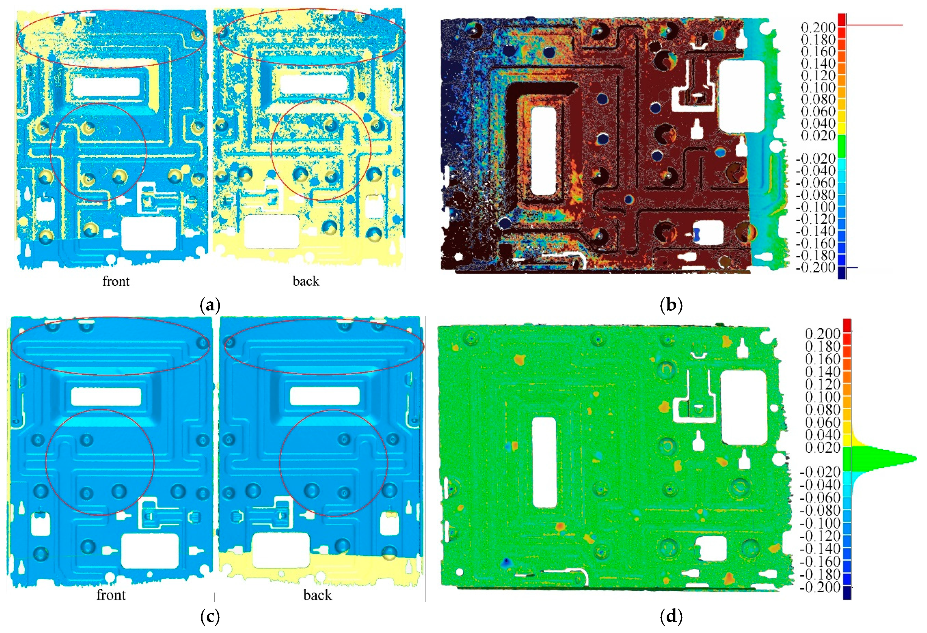
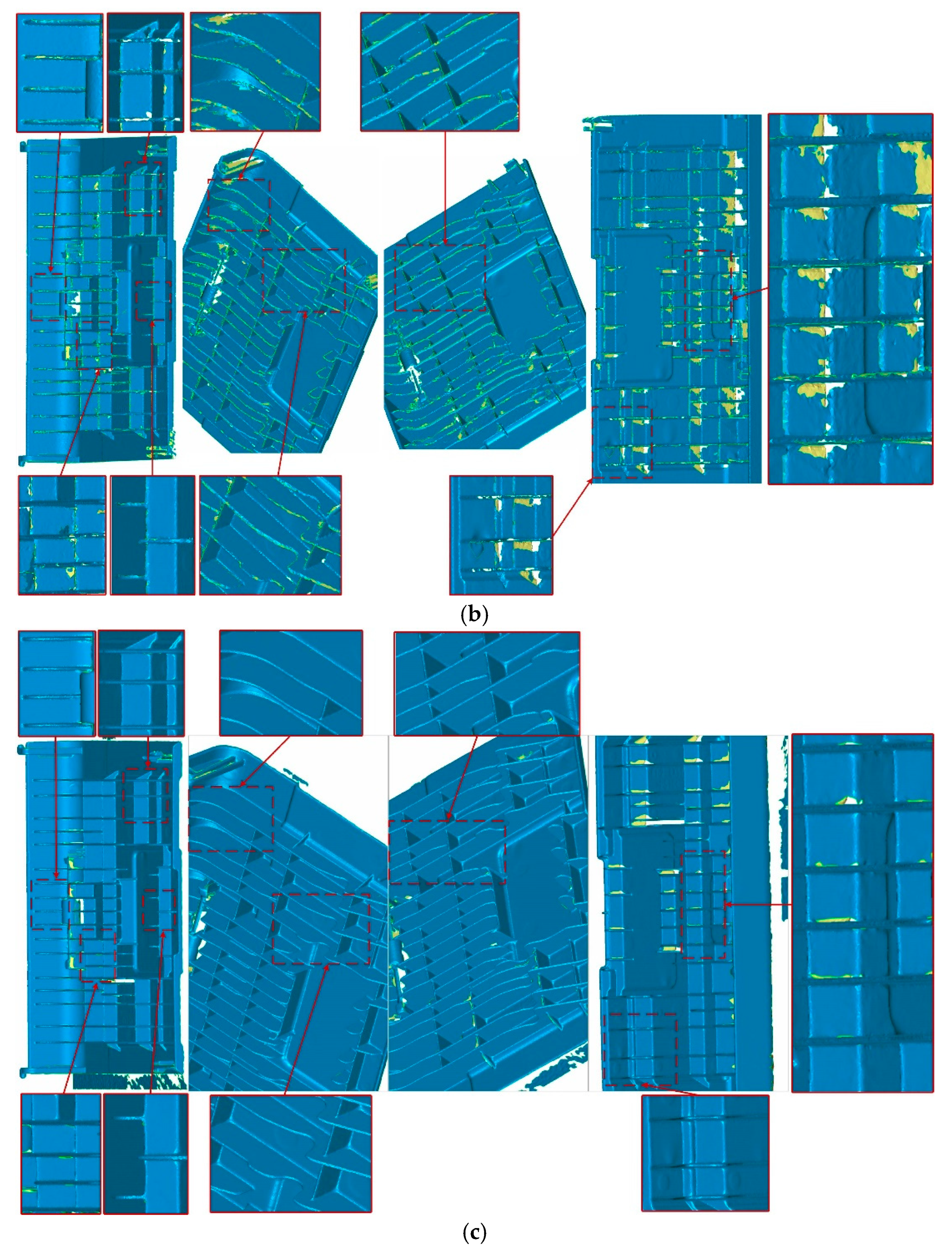
3.2. Qualitative Results
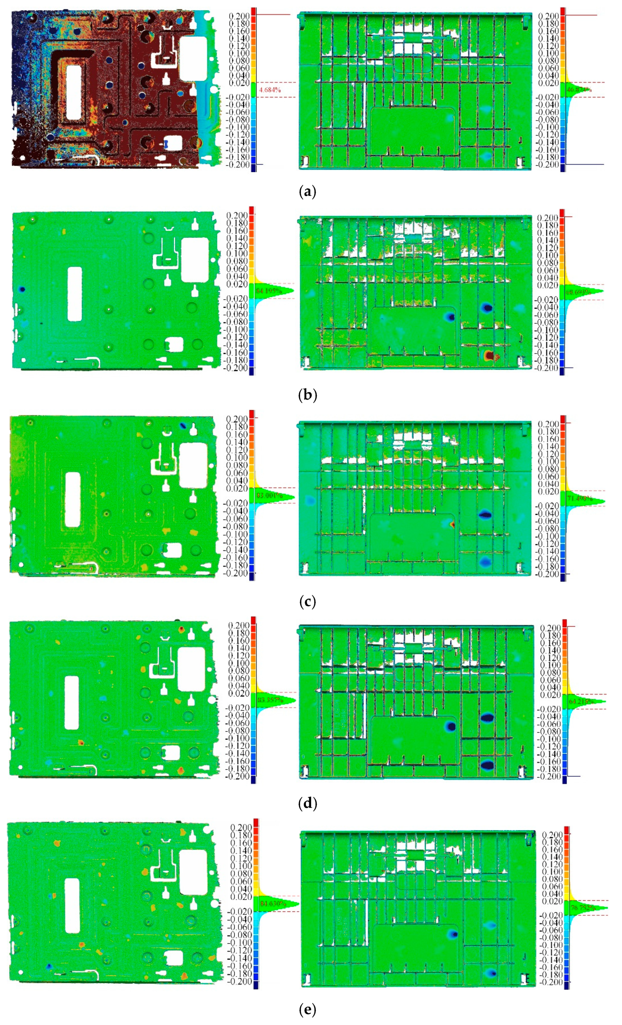
3.3. Quantitative Results
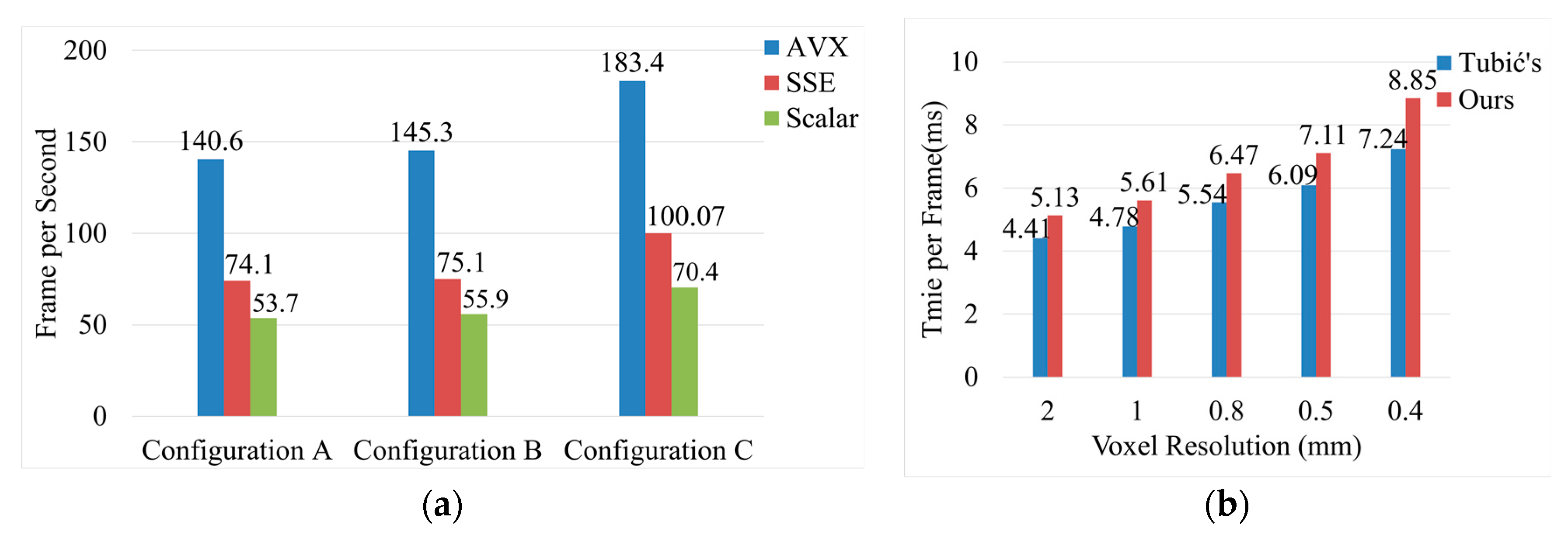
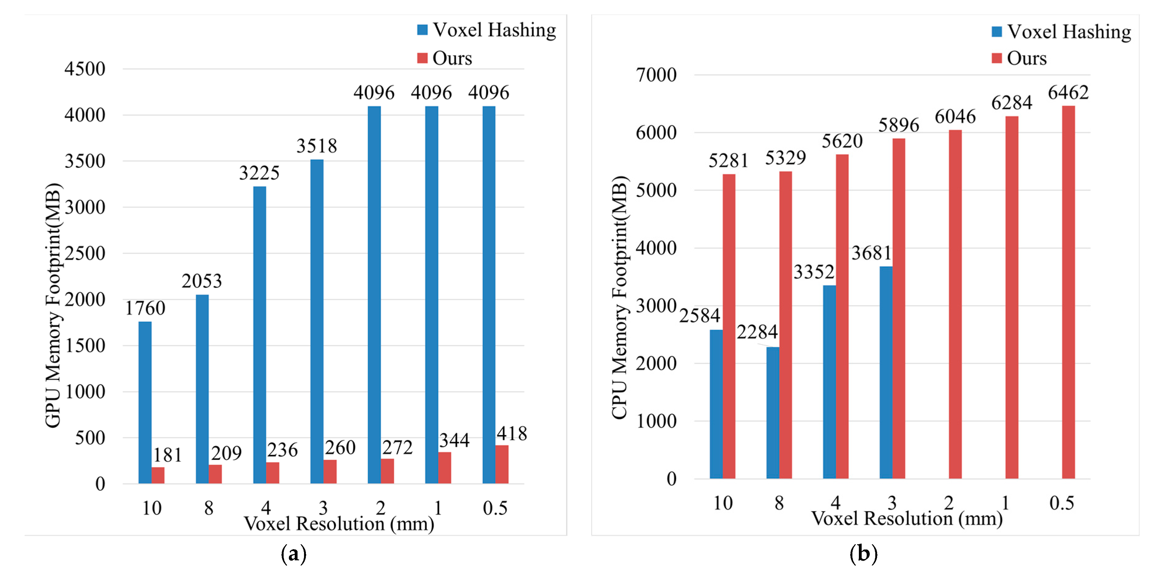
3.4. Performance
3.5. Discussion
4. Conclusions
Author Contributions
Funding
Conflicts of Interest
References
- Kahler, O.; Prisacariu, V.; Valentin, J.; Murray, D. Hierarchical Voxel Block Hashing for Efficient Integration of Depth Images. IEEE Robot. Autom. Lett. 2016, 1, 192–197. [Google Scholar] [CrossRef]
- Bourke, P. Automatic 3D reconstruction: An exploration of the state of the art. GSTF J. Comput. 2018, 2, 71–75. [Google Scholar]
- Henry, P.; Krainin, M.; Herbst, E.; Ren, X.; Fox, D. RGB-D Mapping: Using Depth Cameras for Dense 3D Modeling of Indoor Environments. In Experimental Robotics; Springer: Marrakech, Morocco, 2014; pp. 477–491. [Google Scholar]
- Klingensmith, M.; Dryanovski, I.; Srinivasa, S.; Xiao, J. Chisel: Real Time Large Scale 3D Reconstruction Onboard a Mobile Device using Spatially Hashed Signed Distance Fields. In Proceedings of the Robotics: Science and Systems (RSS), Rome, Italy, 13–17 July 2015. [Google Scholar]
- Lachat, E.; Macher, H.; Landes, T.; Grussenmeyer, P. Assessment and calibration of a RGB-D camera (Kinect v2 Sensor) towards a potential use for close-range 3D modeling. Remote Sens.-Basel 2015, 7, 13070–13097. [Google Scholar] [CrossRef] [Green Version]
- Tubić, D.; Hébert, P.; Laurendeau, D. 3D surface modeling from curves. Image Vis. Comput. 2004, 22, 719–734. [Google Scholar] [CrossRef]
- HandySCAN. Available online: https://www.creaform3d.com/en/portable-3d-scanner-handyscan-3d (accessed on 25 October 2019).
- HSCAN. Available online: https://www.3d-scantech.com/product/hscan771-3d-scanner/ (accessed on 25 October 2019).
- FreeScan. Available online: https://www.shining3d.com/solutions/freescan-x7 (accessed on 25 October 2019).
- Zollhöfer, M.; Stotko, P.; Görlitz, A.; Theobalt, C.; Nießner, M.; Klein, R.; Kolb, A. State of the Art on 3D Reconstruction with RGB-D Cameras. Comput. Graphics Forum 2018, 37, 625–652. [Google Scholar] [CrossRef]
- Hinzmann, T.; Schönberger, J.L.; Pollefeys, M.; Siegwart, R. Mapping on the Fly: Real-Time 3D Dense Reconstruction, Digital Surface map and Incremental Orthomosaic Generation for Unmanned Aerial Vehicles. In Field and Service Robotics; Springer: Zurich, Switzerland, 2018; pp. 383–396. [Google Scholar]
- Cao, Y.; Kobbelt, L.; Hu, S. Real-time High-accuracy Three-Dimensional Reconstruction with Consumer RGB-D Cameras. ACM Trans. Graph. 2018, 37, 171. [Google Scholar] [CrossRef] [Green Version]
- Rusinkiewicz, S.; Levoy, M. Efficient Variants of the ICP Algorithm. In Proceedings of the Third International Conference on 3-D Digital Imaging and Modeling, Quebec, QC, Canada, 28 May–1 June 2001; pp. 145–152. [Google Scholar]
- Stückler, J.; Behnke, S. Integrating Depth and Color Cues for Dense Multi-Resolution Scene Mapping Using Rgb-d Cameras. In Proceedings of the 2012 IEEE Conference on Multisensor Fusion and Integration for Intelligent Systems (MFI), Hamburg, Germany, 13–15 September 2012; pp. 162–167. [Google Scholar]
- Weise, T.; Wismer, T.; Leibe, B.; Van Gool, L. In-Hand Scanning with Online Loop Closure. In Proceedings of the 2009 IEEE 12th International Conference on Computer Vision Workshops (ICCV Workshops), Kyoto, Japan, 29 September–2 October 2009; pp. 1630–1637. [Google Scholar]
- Gallup, D.; Pollefeys, M.; Frahm, J. 3D Reconstruction Using an n-Layer Heightmap. In Joint Pattern Recognition Symposium; Springer: Berlin/Heidelberg, Germany, 2010; pp. 1–10. [Google Scholar]
- Pollefeys, M.; Nistér, D.; Frahm, J.; Akbarzadeh, A.; Mordohai, P.; Clipp, B.; Engels, C.; Gallup, D.; Kim, S.; Merrell, P. Detailed real-time urban 3D reconstruction from video. Int. J. Comput. Vis. 2008, 78, 143–167. [Google Scholar] [CrossRef]
- Izadi, S.; Kim, D.; Hilliges, O.; Molyneaux, D.; Newcombe, R.; Kohli, P.; Shotton, J.; Hodges, S.; Freeman, D.; Davison, A.; et al. KinectFusion: Real-Time 3D Reconstruction and Interaction Using a Moving Depth Camera. In Proceedings of the 24th Annual ACM Symposium on User Interface Software and Technology, Minneapolis, MN, USA, 20–23 October 2011; pp. 559–568. [Google Scholar]
- Kähler, O.; Prisacariu, V.A.; Murray, D.W. Real-Time Large-Scale Dense 3D Reconstruction with Loop Closure. In Proceedings of the European Conference on Computer Vision, Amsterdam, The Netherlands, 8–16 October 2016; pp. 500–516. [Google Scholar]
- Nießner, M.; Zollhöfer, M.; Izadi, S.; Stamminger, M. Real-time 3D reconstruction at scale using voxel hashing. ACM Trans. Graph. 2013, 32, 169. [Google Scholar] [CrossRef]
- Curless, B.; Levoy, M. A Volumetric Method for Building Complex Models from Range Images. In Proceedings of the 23rd Annual Conference on Computer Graphics and Interactive Techniques, New Orleans, LA, USA, 4–9 August 1996; pp. 303–312. [Google Scholar]
- Fedkiw, S.O.R.; Osher, S. Level set methods and dynamic implicit surfaces. Surfaces 2002, 44, 77. [Google Scholar]
- Lorensen, W.E.; Cline, H.E. Marching Cubes: A High Resolution 3D Surface Construction Algorithm. In Proceedings of the 14th annual Conference on Computer graphics and Interactive Techniques, Anaheim, CA, USA, 27–31 July 1987; pp. 163–169. [Google Scholar]
- Kähler, O.; Prisacariu, V.A.; Ren, C.Y.; Sun, X.; Torr, P.; Murray, D. Very high frame rate volumetric integration of depth images on mobile devices. IEEE Trans. Vis. Comput. Graph. 2015, 21, 1241–1250. [Google Scholar] [CrossRef]
- Newcombe, R.A.; Fox, D.; Seitz, S.M. Dynamicfusion: Reconstruction and Tracking of Non-Rigid Scenes in Real-Time. In Proceedings of the IEEE Conference on Computer Vision and Pattern Recognition, Boston, MA, USA, 7–12 June 2015; pp. 343–352. [Google Scholar]
- Bylow, E.; Sturm, J.; Kerl, C.; Kahl, F.; Cremers, D. Real-Time Camera Tracking and 3D Reconstruction Using Signed Distance Functions. In Proceedings of the Robotics: Science and Systems (RSS), Berlin, Germany, 24–28 June 2013. [Google Scholar]
- Dong, W.; Wang, Q.; Wang, X.; Zha, H. PSDF Fusion: Probabilistic Signed Distance Function for On-the-fly 3D Data Fusion and Scene Reconstruction. In Proceedings of the European Conference on Computer Vision (ECCV), Munich, Germany, 8–14 September 2018; pp. 701–717. [Google Scholar]
- Choe, G.; Park, J.; Tai, Y.; Kweon, I.S. Refining geometry from depth sensors using IR shading images. Int. J. Comput. Vis. 2017, 122, 1–16. [Google Scholar] [CrossRef]
- Maier, R.; Kim, K.; Cremers, D.; Kautz, J.; Nießner, M. Intrinsic3d: High-Quality 3D Reconstruction by Joint Appearance and Geometry Optimization with Spatially-Varying Lighting. In Proceedings of the IEEE International Conference on Computer Vision, Honolulu, HI, USA, 21–26 July 2017; pp. 3114–3122. [Google Scholar]
- Zollhöfer, M.; Dai, A.; Innmann, M.; Wu, C.; Stamminger, M.; Theobalt, C.; Nießner, M. Shading-based refinement on volumetric signed distance functions. ACM Trans. Graph. 2015, 34, 96. [Google Scholar] [CrossRef]
- Liu, Y.; Gao, W.; Hu, Z. Geometrically stable tracking for depth images based 3D reconstruction on mobile devices. ISPRS J. Photogramm. 2018, 143, 222–232. [Google Scholar] [CrossRef]
- Slavcheva, M.; Kehl, W.; Navab, N.; Ilic, S. SDF-2-SDF Registration for Real-Time 3D Reconstruction from RGB-D Data. Int. J. Comput. Vis. 2018, 126, 615–636. [Google Scholar] [CrossRef]
- Choi, S.; Zhou, Q.; Koltun, V. Robust Reconstruction of Indoor Scenes. In Proceedings of the IEEE Conference on Computer Vision and Pattern Recognition, Boston, MA, USA, 7–12 June 2015; pp. 5556–5565. [Google Scholar]
- Dai, A.; Nießner, M.; Zollhöfer, M.; Izadi, S.; Theobalt, C. Bundlefusion: Real-time globally consistent 3D reconstruction using on-the-fly surface reintegration. ACM Trans.Graph. 2017, 36, 76a. [Google Scholar] [CrossRef]
- Han, L.; Fang, L. FlashFusion: Real-time Globally Consistent Dense 3D Reconstruction Using CPU Computing. In Proceedings of the Robotics: Science and Systems (RSS), Pittsburgh, PA, USA, 26–30 June 2018. [Google Scholar]
- Maier, R.; Schaller, R.; Cremers, D. Efficient online surface correction for real-time large-scale 3D reconstruction. arXiv 2017, arXiv:1709.03763. [Google Scholar]
- Guo, K.; Taylor, J.; Fanello, S.; Tagliasacchi, A.; Dou, M.; Davidson, P.; Kowdle, A.; Izadi, S. TwinFusion: High Framerate Non-Rigid Fusion Through Fast Correspondence Tracking. In Proceedings of the 2018 International Conference on 3D Vision (3DV), Verona, Italy, 5–8 September 2018; pp. 596–605. [Google Scholar]
- Palazzolo, E.; Behley, J.; Lottes, P.; Giguère, P.; Stachniss, C. ReFusion: 3D Reconstruction in Dynamic Environments for RGB-D Cameras Exploiting Residuals. arXiv 2019, arXiv:1905.02082. [Google Scholar]
- Slavcheva, M.; Baust, M.; Cremers, D.; Ilic, S. Killingfusion: Non-rigid 3D Reconstruction without Correspondences. In Proceedings of the IEEE Conference on Computer Vision and Pattern Recognition, Honolulu, HI, USA, 21–26 July 2017; pp. 1386–1395. [Google Scholar]
- Slavcheva, M.; Baust, M.; Ilic, S. SobolevFusion: 3D Reconstruction of Scenes Undergoing Free Non-Rigid Motion. In Proceedings of the IEEE Conference on Computer Vision and Pattern Recognition, Verona, Italy, 5–8 September 2018; pp. 2646–2655. [Google Scholar]
- Zheng, Z.; Yu, T.; Li, H.; Guo, K.; Dai, Q.; Fang, L.; Liu, Y. Hybrid Fusion: Real-Time Performance Capture Using a Single Depth Sensor and Sparse IMUs. In Proceedings of the European Conference on Computer Vision (ECCV), Munich, Germany, 8–14 September 2018; pp. 384–400. [Google Scholar]
- Riegler, G.; Ulusoy, A.O.; Bischof, H.; Geiger, A. Octnetfusion: Learning Depth Fusion from Data. In Proceedings of the 2017 International Conference on 3D Vision (3DV), Qingdao, China, 10–12 October 2017; pp. 57–66. [Google Scholar]
- Dai, A.; Ritchie, D.; Bokeloh, M.; Reed, S.; Sturm, J.; Nießner, M. Scancomplete: Large-scale scene completion and semantic segmentation for 3D scans. In Proceedings of the IEEE Conference on Computer Vision and Pattern Recognition, Verona, Italy, 5–8 September 2018; pp. 4578–4587. [Google Scholar]
- Chang, A.; Dai, A.; Funkhouser, T.; Halber, M.; Niessner, M.; Savva, M.; Song, S.; Zeng, A.; Zhang, Y. Matterport3d: Learning from rgb-d data in indoor environments. arXiv 2017, arXiv:1709.06158. [Google Scholar]
- Dai, A.; Chang, A.X.; Savva, M.; Halber, M.; Funkhouser, T.; Nießner, M. Scannet: Richly-annotated 3D reconstructions of indoor scenes. In Proceedings of the IEEE Conference on Computer Vision and Pattern Recognition, Honolulu, HI, USA, 21–26 July 2017; pp. 5828–5839. [Google Scholar]
- Hou, J.; Dai, A.; Nießner, M. 3D-sis: 3D Semantic Instance Segmentation of rgb-d Scans. In Proceedings of the IEEE Conference on Computer Vision and Pattern Recognition, Long Beach, CA, USA, 16–20 June 2019; pp. 4421–4430. [Google Scholar]
- McCormac, J.; Clark, R.; Bloesch, M.; Davison, A.; Leutenegger, S. Fusion++: Volumetric Object-Level Slam. In Proceedings of the 2018 International Conference on 3D Vision (3DV), Verona, Italy, 5–8 September 2018; pp. 32–41. [Google Scholar]
- Pham, Q.; Hua, B.; Nguyen, T.; Yeung, S. Real-Time Progressive 3D Semantic Segmentation for Indoor Scenes. In Proceedings of the 2019 IEEE Winter Conference on Applications of Computer Vision (WACV), Waikoloa Village, HI, USA, 7–11 January 2019; pp. 1089–1098. [Google Scholar]
- Vineet, V.; Miksik, O.; Lidegaard, M.; Nießner, M.; Golodetz, S.; Prisacariu, V.A.; Kähler, O.; Murray, D.W.; Izadi, S.; Pérez, P. Incremental Dense Semantic Stereo Fusion for Large-Scale Semantic Scene Reconstruction. In Proceedings of the 2015 IEEE International Conference on Robotics and Automation (ICRA), Seattle, WA, USA, 26–30 May 2015; pp. 75–82. [Google Scholar]
- Whelan, T.; Kaess, M.; Johannsson, H.; Fallon, M.; Leonard, J.J.; McDonald, J. Real-time large-scale dense RGB-D SLAM with volumetric fusion. Int. J. Robot. Res. 2015, 34, 598–626. [Google Scholar] [CrossRef] [Green Version]
- Chen, J.; Bautembach, D.; Izadi, S. Scalable real-time volumetric surface reconstruction. ACM Trans. Graph. 2013, 32, 113. [Google Scholar] [CrossRef]
- Steinbrücker, F.; Sturm, J.; Cremers, D. Volumetric 3D Mapping in Real-Time on a CPU. In Proceedings of the 2014 IEEE International Conference on Robotics and Automation (ICRA), Hong Kong, China, 31 May–7 June 2014; pp. 2021–2028. [Google Scholar]
- Zeng, M.; Zhao, F.; Zheng, J.; Liu, X. Octree-Based Fusion for Realtime 3D Reconstruction. Graph. Models 2013, 75, 126–136. [Google Scholar] [CrossRef]
- Dryanovski, I.; Klingensmith, M.; Srinivasa, S.S.; Xiao, J. Large-scale, real-time 3D scene reconstruction on a mobile device. Auton. Robot. 2017, 41, 1423–1445. [Google Scholar] [CrossRef]
- Li, S.; Cheng, M.; Liu, Y.; Lu, S.; Wang, Y.; Prisacariu, V.A. Structured Skip List: A Compact Data Structure for 3D Reconstruction. In Proceedings of the 2018 IEEE/RSJ International Conference on Intelligent Robots and Systems (IROS), Madrid, Spain, 1–5 October 2018; pp. 1–7. [Google Scholar]
- França, J.G.D.; Gazziro, M.A.; Ide, A.N.; Saito, J.H. A 3D Scanning System Based on Laser Triangulation and Variable Field of View. In Proceedings of the IEEE International Conference on Image Processing 2005, Genova, Italy, 11–14 September 2005; p. 425. [Google Scholar]
- Pauly, M.; Gross, M.; Kobbelt, L.P. Efficient simplification of point-sampled surfaces. In Proceedings of the the conference on Visualization’02, Washington, DC, USA, 2 October 2002; pp. 163–170. [Google Scholar]
- Lu, X.; Wu, S.; Chen, H.; Yeung, S.; Chen, W.; Zwicker, M. GPF: GMM-inspired feature-preserving point set filtering. IEEE Trans. Vis. Comput. Graph. 2018, 24, 2315–2326. [Google Scholar] [PubMed]
- Sharf, A.; Lewiner, T.; Shklarski, G.; Toledo, S.; Cohen-Or, D. Interactive Topology-Aware Surface Reconstruction. ACM Trans. Graphics (TOG) 2007, 26, 43. [Google Scholar] [CrossRef]
- Vaillant, R. Recipe for Implicit Surface Reconstruction with HRBF-Rodolphe Vaillant’s Homepage. Available online: http://rodolphe-vaillant.fr/?e=12 (accessed on 30 August 2019).
- Handa, A.; Whelan, T.; McDonald, J.; Davison, A.J. A Benchmark for RGB-D Visual Odometry, 3D Reconstruction and SLAM. In Proceedings of the 2014 IEEE International Conference on Robotics and Automation (ICRA), Hong Kong, China, 31 May–5 June 2014; pp. 1524–1531. [Google Scholar]
- Welch’s t-Test. Available online: https://en.wikipedia.org/wiki/Welch%27s_t-test (accessed on 8 January 2020).
- F-Test of Equality of Variances. Available online: https://en.wikipedia.org/wiki/F-test_of_equality_of_variances (accessed on 8 January 2020).
- R Programming Language. Available online: https://www.r-project.org/ (accessed on 8 January 2020).
- Pearson’s Chi-Squared Test. Available online: https://en.wikipedia.org/wiki/Pearson%27s_chi-squared_test (accessed on 8 January 2020).
- One-and Two-Tailed Tests. Available online: https://en.wikipedia.org/wiki/One-_and_two-tailed_tests (accessed on 8 January 2020).
- SIMD. Available online: https://en.wikipedia.org/wiki/SIMD (accessed on 8 January 2020).
- Advanced Vector Extensions. Available online: https://en.wikipedia.org/wiki/Advanced_Vector_Extensions (accessed on 8 January 2020).
- Streaming SIMD Extensions. Available online: https://en.wikipedia.org/wiki/Streaming_SIMD_Extensions (accessed on 8 January 2020).


| Scanner | Volumetric Accuracy 1 (Based on Part Size) |
|---|---|
| Creaform HandySCAN700 [7] | 0.020 mm + 0.100 mm/m |
| Scantech HSCAN771 [8] | 0.020 mm + 0.060 mm/m |
| PC | Configuration |
|---|---|
| Configuration A | Intel Core i7-7700HQ (2.8 GHz), 32 GB RAM, NVIDIA GeForce GTX1050 (4 GB) |
| Configuration B | Intel Core i7-7700 (3.6 GHz), 32 GB RAM, NVIDIA GeForce GTX960 (2 GB) |
| Configuration C | Intel Core i7-7820X (3.6 GHz), 128 GB RAM, NVIDIA GeForce GTX1060 (4 GB) |
| Object | Tubić et al. [6] | Creaform [7] | Scantech [8] | Our Real-Time Approach | Our Post-Processing Approach |
|---|---|---|---|---|---|
| sheet metal part | 0.1559 ± 0.2592 (544,565) 1 | −0.0010 ± 0.0750 (1,135,616) | 0.0024 ± 0.0408 (620,037) | −0.0011 ± 0.0227 (680,628) | −0.0005 ± 0.0212 (681,574) |
| plastic shell | 0.0093 ± 0.2412 (443,417) | 0.0015 ± 0.0913 (441,490) | −0.0053 ± 0.0554 (439,817) | −0.0045 ± 0.0768 (458,489) | −0.0008 ± 0.0379 (489,797) |
| Object | Tubić et al. [6] | Creaform [7] | Scantech [8] | Our Real-Time Approach | Our Post-Processing Approach |
|---|---|---|---|---|---|
| sheet metal part | 0.1589 ± 0.2660 | −0.0010 ± 0.0737 | 0.0031 ± 0.0439 | −0.0012 ± 0.0231 | −0.0011 ± 0.0220 |
| plastic shell | 0.0071 ± 0.2727 | 0.0039 ± 0.1080 | −0.0041 ± 0.0691 | −0.0032 ± 0.0922 | −0.0012 ± 0.0431 |
| Object | Tubić et al. [6] | Creaform [7] | Scantech [8] | Our Real-Time Approach | Our Post-Processing Approach |
|---|---|---|---|---|---|
| sheet metal part | 0.8562 (3.2968, 7) 1 | 0.3485 (7.8224, 7) | 0.5507 (5.9062, 7) | 0.7404 (5.1586, 8) | 0.6724 (5.7747, 8) |
| plastic shell | 0.9396 (2.9140, 8) | 0.5922 (4.6288, 6) | 0.9076 (3.3884, 8) | 0.4392 (6.9007, 7) | 0.4480 (7.8516,8) |
| Tubić et al. [6] | Creaform [7] | Scantech [8] | Our Real-Time Approach | |
|---|---|---|---|---|
| Creaform [7] | 0.0 * (18.0343, 1151) 1 | |||
| Scantech [8] | 0.0 * (18.2162, 1053) | 0.7816 (−7.7813, 1628) | ||
| Our Real-time Approach | 0.0 * (18.6183, 1014) | 0.5343 (−0.0862, 1194) | 0.1131 (1.2105, 1514) | |
| Our Post-processing Approach | 0.0 * (18.6405, 1012) | 0.5131 (−0.0330, 1175) | 0.0956 (1.3072, 1471) | 0.4487 (0.1288, 1992) |
| Tubić et al. [6] | Creaform [7] | Scantech [8] | Our Real-Time Approach | |
|---|---|---|---|---|
| Creaform [7] | 0.0 * (7.2831, 1305) 1 | |||
| Scantech [8] | 0.0 * (7.5697, 1126) | 0.5210 (−0.5275, 1699) | ||
| Our Real-time Approach | 0.0 * (7.4946, 1224) | 0.4410 (0.1483, 1949) | 0.4045 (0.2416, 1852) | |
| Our Post-processing Approach | 0.0 * (8.0481, 1049) | 0.2307 (7.3644, 1309) | 0.1284 (1.1343, 1675) | 0.2628 (0.63468, 1416) |
| Tubić et al. [6] | Creaform [7] | Scantech [8] | Our Real-Time Approach | |
|---|---|---|---|---|
| Creaform [7] | 0.0 * (13.0255) 1 | |||
| Scantech [8] | 0.0 * (36.6872) | 0.0 * (2.8165) | ||
| Our Real-time Approach | 0.0 * (132.0038) | 0.0 * (10.1342) | 0.0 * (3.5980) | |
| Our Post-processing Approach | 0.0 * (146.0340) | 0.0 * (11.2113) | 0.0 * (3.9805) | 0.0553 (1.1062) |
| Tubić et al. [6] | Creaform [7] | Scantech [8] | Our Real-Time Approach | |
|---|---|---|---|---|
| Creaform [7] | 0.0 * (6.3688) 1 | |||
| Scantech [8] | 0.0 * (15.5554) | 0.0 * (2.4424) | ||
| Our Real-time Approach | 0.0 * (8.7480) | 2.8 × 10−7 * (1.3735) | 1.0 (0.56237) | |
| Our Post-processing Approach | 0.0 * (39.9106) | 0.0 * (6.2665) | 0.0 * (2.5656) | 0.0 * (4.5622) |
© 2020 by the authors. Licensee MDPI, Basel, Switzerland. This article is an open access article distributed under the terms and conditions of the Creative Commons Attribution (CC BY) license (http://creativecommons.org/licenses/by/4.0/).
Share and Cite
He, Y.; Zheng, S.; Zhu, F.; Huang, X. Real-Time 3D Reconstruction of Thin Surface Based on Laser Line Scanner. Sensors 2020, 20, 534. https://doi.org/10.3390/s20020534
He Y, Zheng S, Zhu F, Huang X. Real-Time 3D Reconstruction of Thin Surface Based on Laser Line Scanner. Sensors. 2020; 20(2):534. https://doi.org/10.3390/s20020534
Chicago/Turabian StyleHe, Yuan, Shunyi Zheng, Fengbo Zhu, and Xia Huang. 2020. "Real-Time 3D Reconstruction of Thin Surface Based on Laser Line Scanner" Sensors 20, no. 2: 534. https://doi.org/10.3390/s20020534
APA StyleHe, Y., Zheng, S., Zhu, F., & Huang, X. (2020). Real-Time 3D Reconstruction of Thin Surface Based on Laser Line Scanner. Sensors, 20(2), 534. https://doi.org/10.3390/s20020534