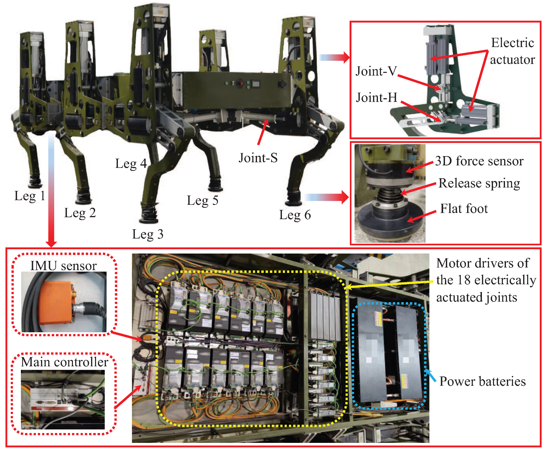
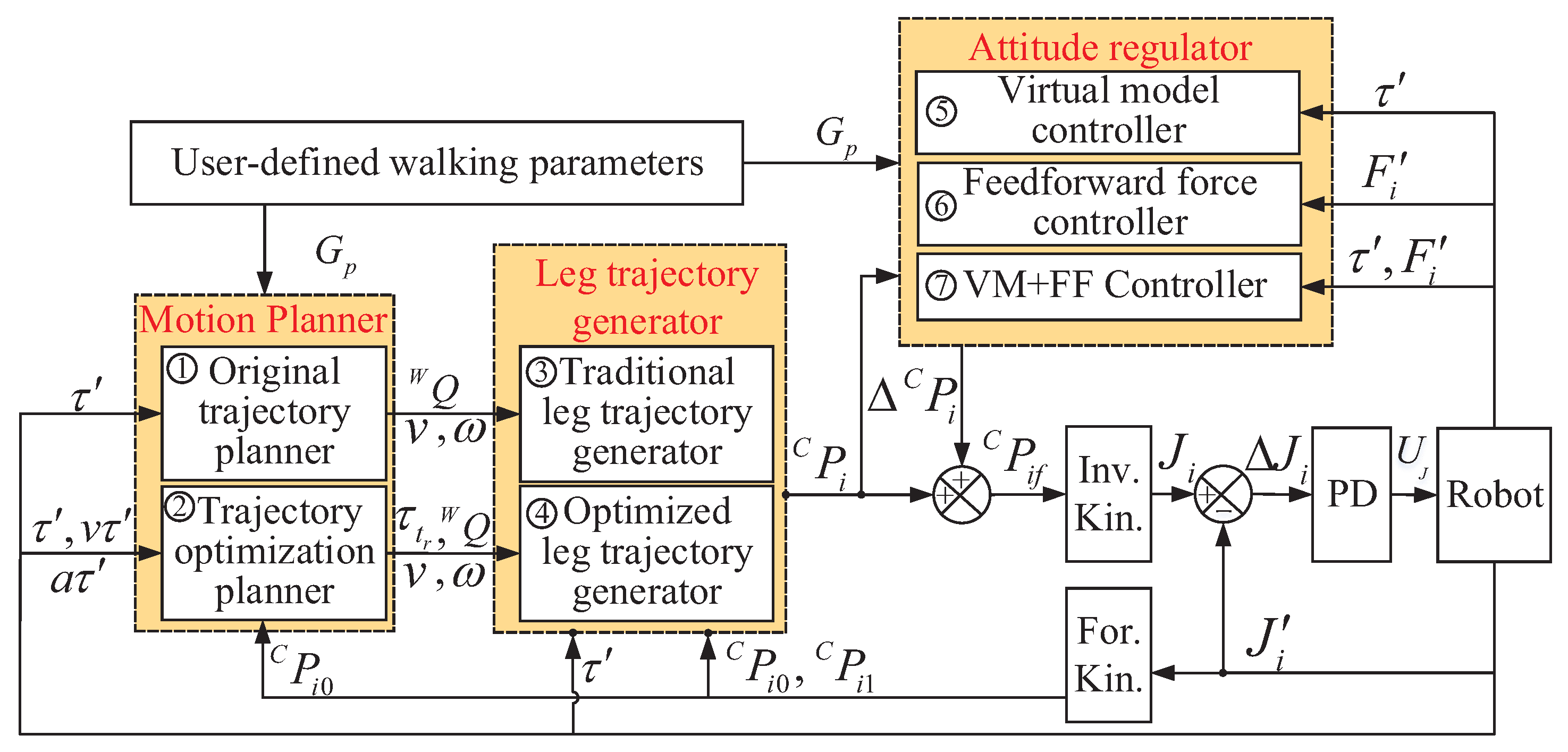
3.2.1. Swing Leg Trajectory Generation
As discussed in the introduction, for most currently developed legged robots, the swing leg trajectory is usually designed in the body coordinate
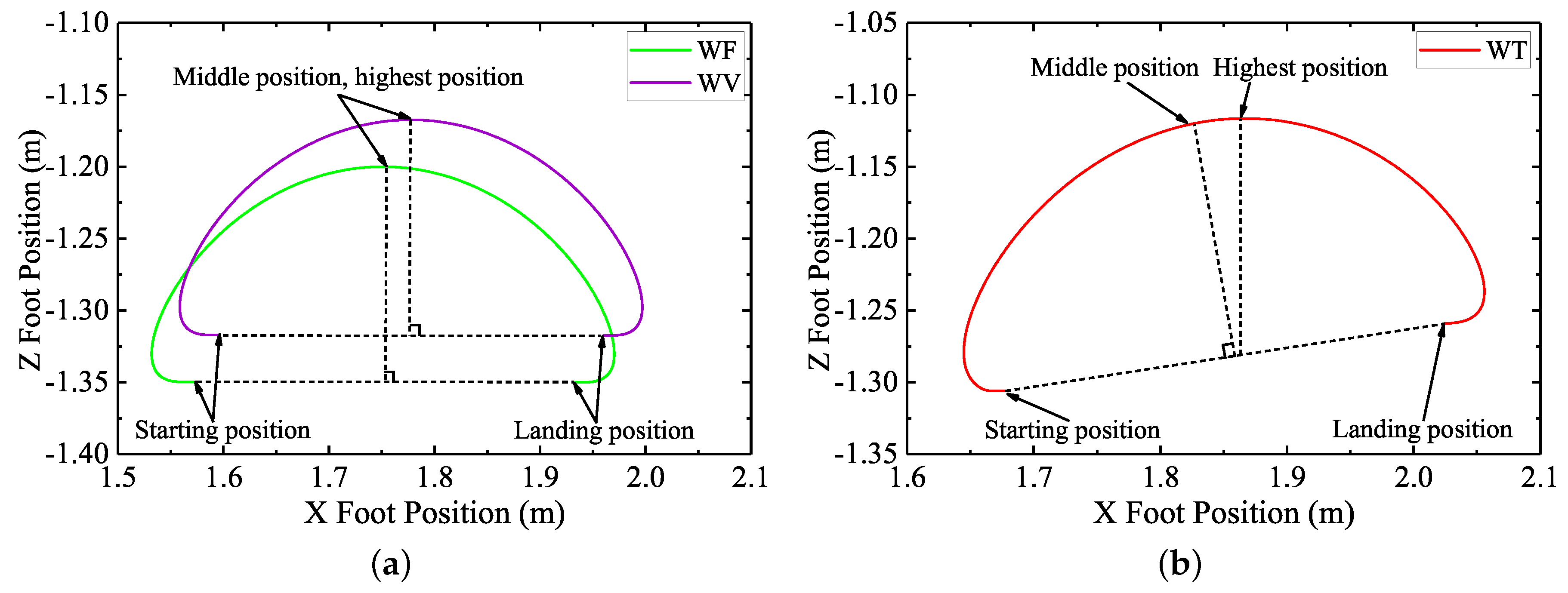
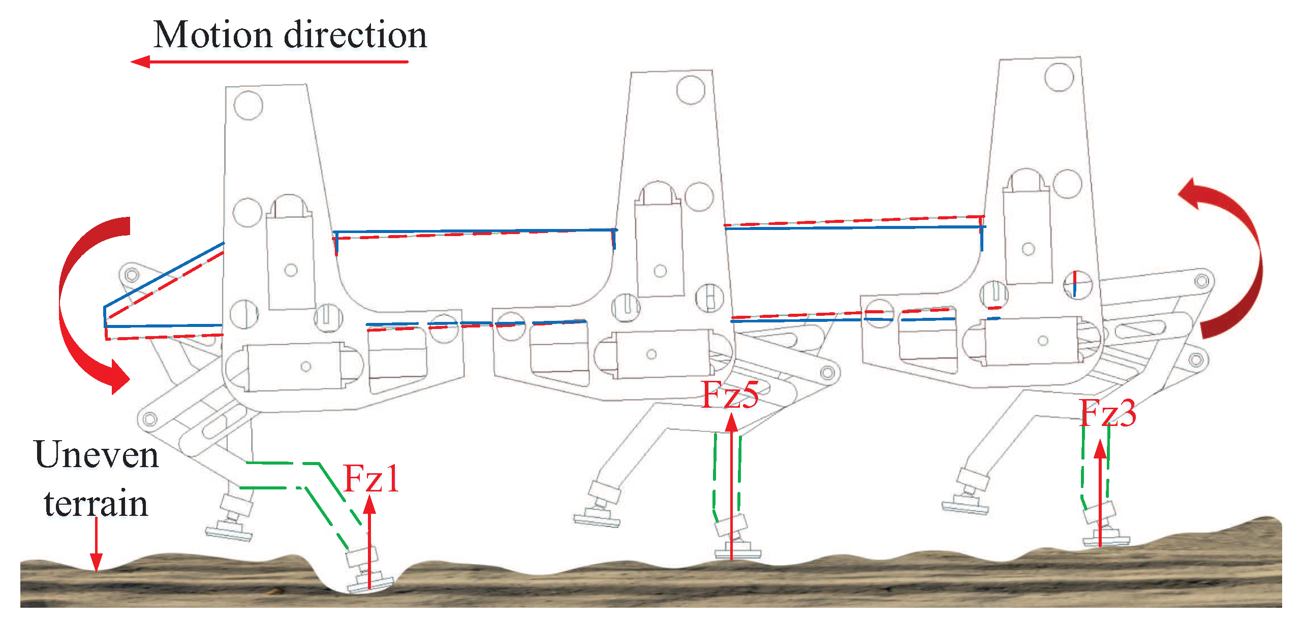
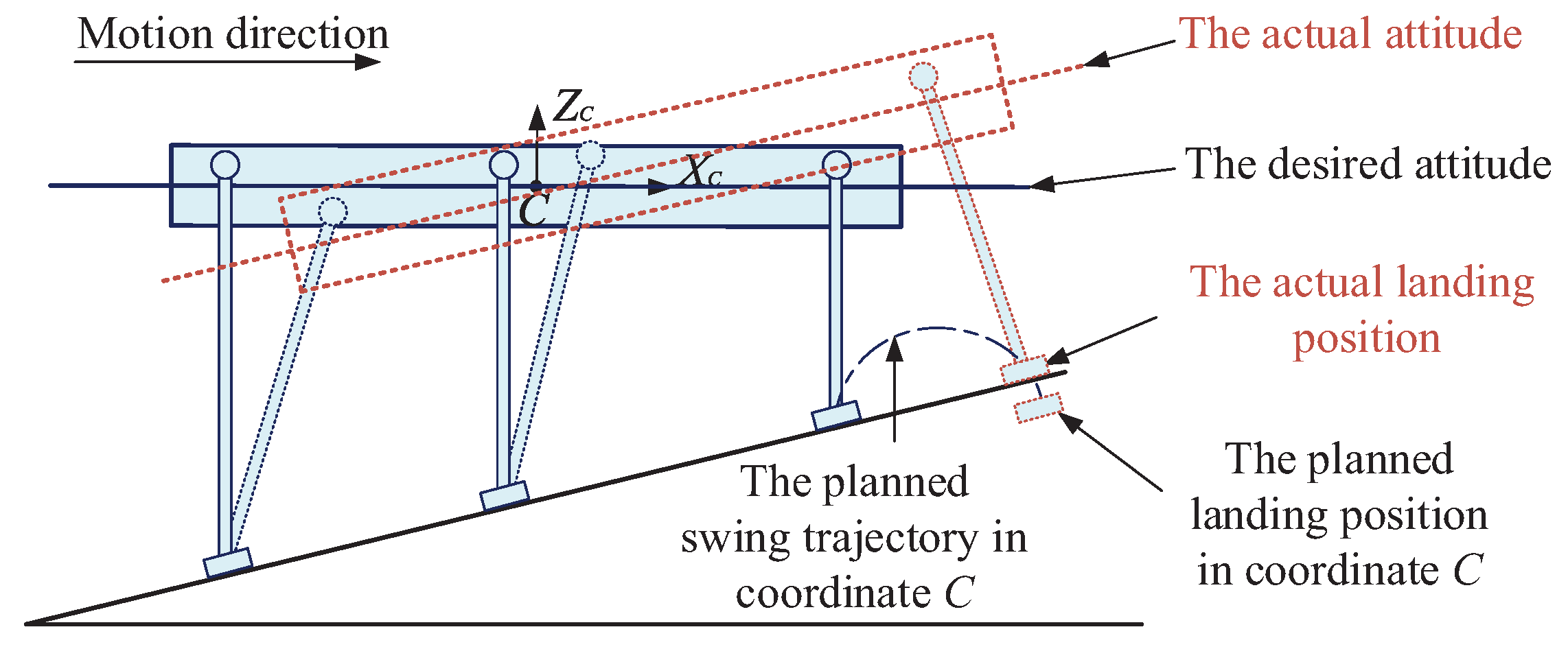
C without considering the terrain attitude angles. When facing the slope walking situation, the early landings of the swing legs may occur. The swing legs with the unchangeable landing positions with respect to the robot body coordinate
C will keep moving to the planned landing positions and force the robot body to be parallel to the slope surface. Therefore, the attitude adjustment process with special user-defined desired attitude angles will be hindered. The contradiction between the unchangeable landing positions of the swing legs and the attitude adjustment process will further affect the motion balance of the robot, as shown in
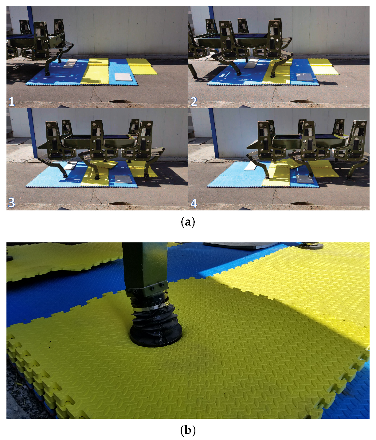
Figure 6.
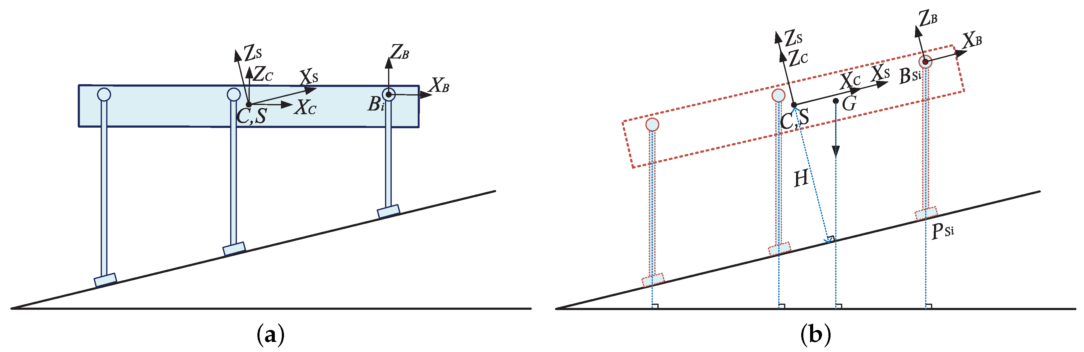
To solve this problem, a swing leg trajectory generation method with terrain attitude angles considered is proposed. For a slope-climbing legged robot, the attitude angles of the slope are important factors which will influence the walking balance of the robot. Therefore, to get a swing leg trajectory which can adapt to the terrain, the slope attitude angles are needed to be obtained first. Similar to the coordinates defined in the authors’ previous work [
35] (see Figure 3 in reference [
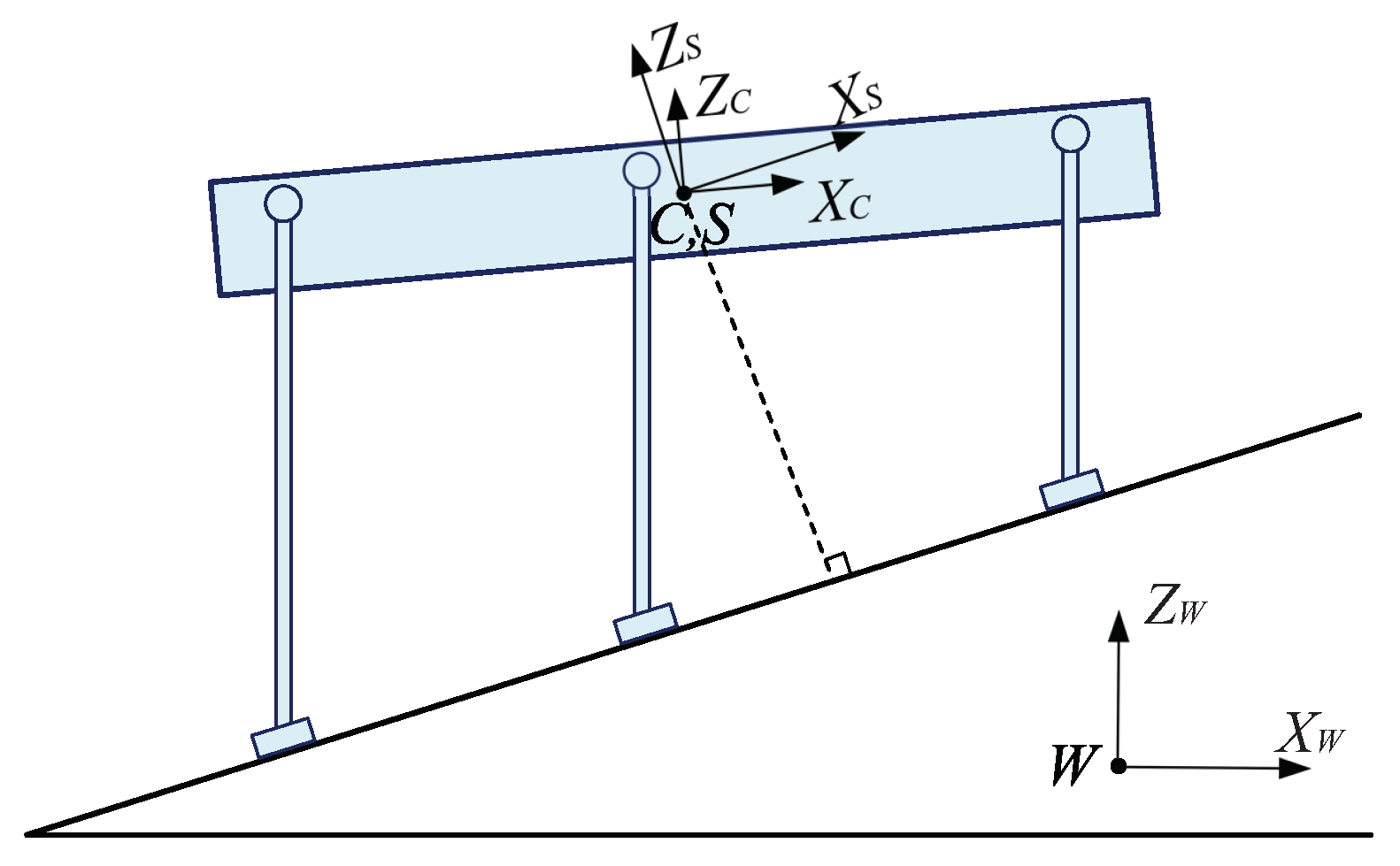
35]), a slope coordinate
S and the global coordinate
W are defined to obtain the slope attitude angles, as shown in
Figure 7. The origin of the slope coordinate
S is located at the origin of the body coordinate
C. The
z-axis of coordinate
S, namely the
-axis shown in
Figure 7, is defined to be perpendicular to the slope surface. The
x-axis of coordinate
S, namely the
-axis shown in
Figure 7, is defined to be parallel to the slope surface. The yaw angle of the slope is defined as the same as the yaw angle of the robot. The
z-axis of the global coordinate
W, namely the
-axis shown in
Figure 7, is defined to be perpendicular to the horizontal plane. The
x-axis of coordinate
W, namely the
-axis shown in
Figure 7, is defined to be parallel to the horizontal plane with the same direction as the initial
x-direction of coordinate
C. The
y-axis of coordinate
W is defined to be perpendicular to axis
and axis
, with the same direction as the initial
y-direction of coordinate
C. The coordinate
W is an absolute coordinate and can be located anywhere according to the robot users’ commands.
In the authors’ previous work [
35], a macro terrain recognition method is proposed to obtain the slope plane based on the foot positions of the support legs. Through the macro terrain recognition method, the unit normal vector of the slope
=
can be calculated using Equation (
4) shown in [
35]. Employing the same
in reference [
35], the relationship between
=
which represents the unit normal vector of the global coordinate
W, and
can be obtained, as shown in Equation (
20):
where
represents the rotation transformation matrix of the slope coordinate
S with respect to the global coordinate
W.
has the same form as
shown in Equation (
10), and consists of the actual yaw angle
, the actual pitch angle
, and the actual roll angle
of the slope coordinate
S.
During walking, the actual yaw angles of the body coordinate
C and the slope coordinate
S are the same. Based on this, by solving Equation (
20), the attitude angles of the slope coordinate
S can be obtained, as shown in Equation (
21):
where
represents the actual yaw angle of the robot during walking.
During a slope-climbing process, if a special body attitude of the hexapod robot is wanted to be ensured instead of being parallel to the slope surface at any time, the swing leg trajectory should be designed in the slope coordinate S to reduce the risk of lifting up the body. However, the swing leg trajectory must be finally generated through the inverse kinematics computations, and the inverse kinematics model of the robot is defined in the body coordinate C. Therefore, theoretically, the swing leg trajectory should be designed in the body coordinate C. To solve this conflict, assuming that the robot body is parallel to the slope. Based on this assumption, the swing leg trajectory designed in the slope coordinate S is the same as that in the body coordinate C. Then, combined with the actual attitude angles of the slope and the body, the swing leg trajectory can be transformed from the slope coordinate S to the actual body coordinate C.
To achieve a smooth trajectory of the swing leg, and reduce the velocity change brought by the leg status switching, a similar 6-order polynomial interpolation method to the attitude trajectory planning process is employed to design the swing leg trajectory in the slope coordinate
S, as shown in Equation (
22):
where
,
,
,
,
,
, and
represent the polynomial parameters which need to be determined.
r represents the direction of the slope coordinate
S, and
r can be
x,
y, or
z.
Based on Equation (
22), the velocity trajectory and acceleration trajectory of the swing leg along the
r-direction of the slope coordinate
S can be obtained, as shown in Equations (23) and (24), respectively.
To obtain the unknown polynomial parameters and generate the swing leg trajectory, seven trajectory parameters of the swing leg should be designed, which are the starting position, velocity, and acceleration of the foot at the time
, the landing position, velocity, and acceleration of the foot at the time
, and the middle position of the foot at the time
. Based on the seven trajectory parameters and their corresponding times, the unknown polynomial parameters can be computed, as shown in Equation (
25):
where
,
and
represent the starting foot position, velocity, and acceleration of the swing leg trajectory along the
r-direction of the slope coordinate
S, respectively.
,
and
represent the landing foot position, velocity, and acceleration of the swing leg trajectory along the
r-direction of coordinate
S, respectively.
represents the middle foot position of the swing leg trajectory along the
r-direction of coordinate
S.
The starting foot position of a swing leg is the ending foot position of the same support leg. Therefore, based on the actual ending joint positions of the support leg
i, the actual starting foot position of the swing leg
i at the time
in the body coordinate
C can be obtained through the computation of Equation (
1). Then, the starting foot position of the swing leg
i in the slope coordinate
S can be obtained, as shown in Equation (
26):
where
represents the starting foot position vector of the swing leg
i in the body coordinate
C at the time
.
represents the rotation transformation matrix of the body coordinate
C with respect to the global coordinate
W.
has the same form as
shown in Equation (
10), and consists of the actual yaw, pitch, and roll angles of the robot during walking.
represents the starting foot position vector of the swing leg
i in the slope coordinate
S at the time
.
Based on
,
which represents the starting foot velocity of the swing leg
i, and
, which represents the starting foot acceleration of the swing leg
i can be computed using the differential method, as shown in Equation (
27):
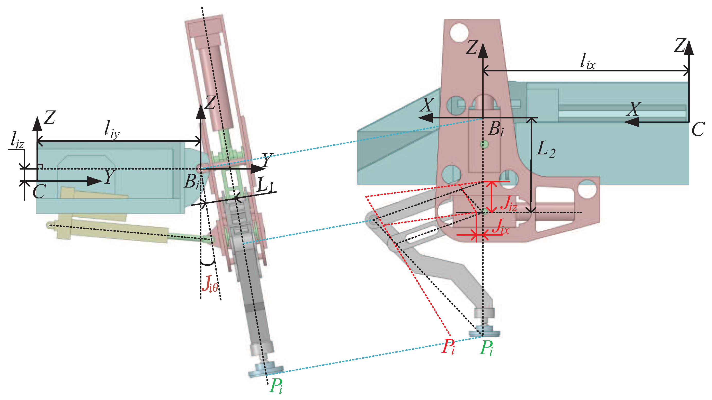
To obtain the landing foot position, velocity, and acceleration of the swing leg, a hypothetical foot position of a support leg relative to the robot body when the robot is standing still is designed first. Assuming that the robot body is parallel to the slope when the robot is standing still on the slope, a hypothetical base coordinate
of leg
i with the same directions as the slope coordinate can be obtained, as shown in
Figure 8b. At this moment, when the line between the foot and the hypothetical base coordinate of the leg is parallel to the direction of the gravity, the projection of the CoM of the robot body in the polygon formed by the support feet is close to the center of the support polygon, and better stability of the robot can be ensured. Based on this hypothetical posture of the robot, the foot position of leg
i in coordinate
can be obtained, as shown in Equation (
28):
where
k represents the equivalent leg length.
represents the foot position vector of leg
i in coordinate
.
The robot body height
H is usually set by the robot users; therefore,
can be calculated as shown in Equation (
29):
By substituting Equation (
29) into Equation (
28),
and
can be calculated, as shown in Equation (
30):
Due to the existing distance
between the hypothetical base coordinate and the plane of the parallelogram mechanism of the leg,
needs to be updated according to the actual robot structure, as shown in Equation (
31):
Under the hypothetical posture of the robot, the robot body coordinate
C is the same as the slope coordinate
S. Therefore, based on Equation (
3), the hypothetical foot position of leg
i in the slope coordinate
S can be obtained, as shown in Equation (
32):
where
represents the hypothetical foot position vector of leg
i in the slope coordinate
S when the robot is standing still on the slope.
To maintain as high stability as possible at any time during walking,
should be kept in the middle position of a step. Therefore, based on the robot step lengths and steering angle set by the robot users, the landing foot position of the swing leg
i can be obtained, as shown in Equation (
33):
where
represents the landing foot position vector of the swing leg
i in coordinate
S.
and
represent the step lengths along the
x- and
y-directions of the slope coordinate
S which are set by the robot users during walking.
represents the steering angle of the robot set by the robot users. For a straight walking process,
and
are set to zero.
Based on the landing foot position of the swing leg
i calculated, and the walking parameters set by the robot users, the landing foot velocity of the swing leg
i can be obtained, as shown in Equation (
34):
with
where
represents the landing foot velocity vector of the swing leg
i in coordinate
S.
represents the translational velocity vector of the robot body in coordinate
S.
represents the angular velocity of the robot body.
The landing foot acceleration of the swing leg
i can be calculated using the differential method, as shown in Equation (
36):
For a swing leg, the step height
h is usually set by the robot users before walking. Then, based on the step height, the starting foot position and landing foot position of the swing leg
i calculated, the middle foot position can be obtained, as shown in Equation (
37):
where
represents the middle foot position vector of the swing leg
i in coordinate
S.
Based on
from Equation (
26),
and
from Equation (
27),
from Equation (
33),
from Equation (
34),
from Equation (
36), and
from Equation (
37), the unknown polynomial parameters in Equation (
25) can be calculated. Based on the polynomial parameters calculated, the swing leg trajectory of leg
i in coordinate
S can be finally obtained using Equation (
22). Then, considering the actual body attitude, the swing leg trajectory of leg
i in the body coordinate
C can be easily obtained, as shown in Equation (
38):
By using the inverse kinematics model shown in Equation (
2), the joint trajectories which satisfy the swing leg trajectory of leg
i designed can be calculated. Then, with the motions of the joints, the actual swing leg trajectory of leg
i with both the body attitude angles and the terrain attitude angles considered can be finally generated.
3.2.2. Support Leg Trajectory Generation
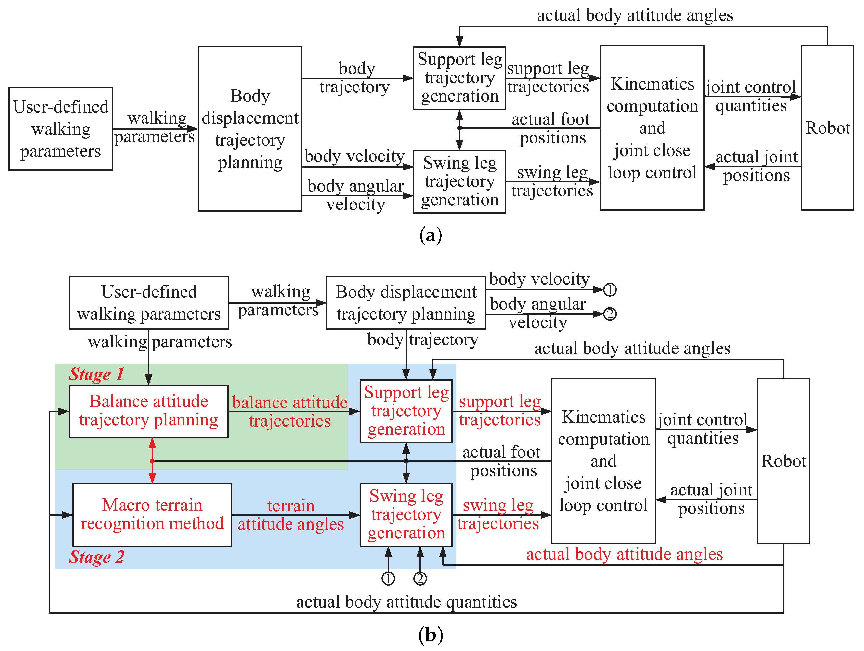
For the balance locomotion generation of a legged creature, the destination, moving velocity, and body posture may be firstly determined. Then, the motions of the support legs to keep the body balance are generated automatically by the central nervous system. Namely, to generate the motions of the support legs, the body displacement trajectory, and the body attitude trajectories should be defined first. The attitude trajectories can be planned through the balance attitude trajectory planning process, so the critical point to generate the support leg trajectory is to obtain the body displacement trajectory.
Based on the gait parameters set by the robot users, the body moving velocities along different directions of the slope coordinate
S can be obtained through the computation of Equation (
35). Then, based on the actual attitude angles of the slope, the global moving velocity vector
of the robot can be obtained, as shown in Equation (
39):
During every attitude adjustment cycle, the global body displacement trajectory of the robot can be calculated by integrating the global moving velocity in the adjustment time, as shown in Equation (
40):
where
represents the global body displacement vector of the robot during one attitude adjustment cycle.
During every attitude adjustment cycle, the robot body and the support legs together can be treated as a parallel mechanism. At the beginning time of an attitude adjustment cycle, namely at time
, the origin of the body coordinate
C is defined as the origin of the global coordinate
W. Therefore, based on the initial body attitude angles at the time
obtained by the IMU feedback signals, the foot position of the support leg
i at time
in the global coordinate
W can be obtained, as shown in Equation (
41):
where
represents the foot position of leg
i in the global coordinate at the time
.
As the robot can be treated as a parallel mechanism,
can be treated as the fixed platform position of the parallel mechanism. Therefore, during one attitude adjustment cycle, the desired support trajectory of leg
i to ensure the walking balance of the robot in the body coordinate
C can be obtained based on the inverse kinematics computation of the parallel mechanism, the planned attitude trajectories, and the body displacement trajectory, as shown in Equation (
42):
where
represents the the planned rotation transformation matrix of the body coordinate
C with respect to the global coordinate
W.
has the same form as
shown in Equation (
10), and consists of the balance yaw, pitch, and roll trajectories planned in Equation (
4).
It can be seen from Equation (
42) that the support trajectory of leg
i is automatically generated according to the planned balance body attitude trajectories. Then, based on Equations (2) and (3), the joint trajectories of leg
i can be computed.
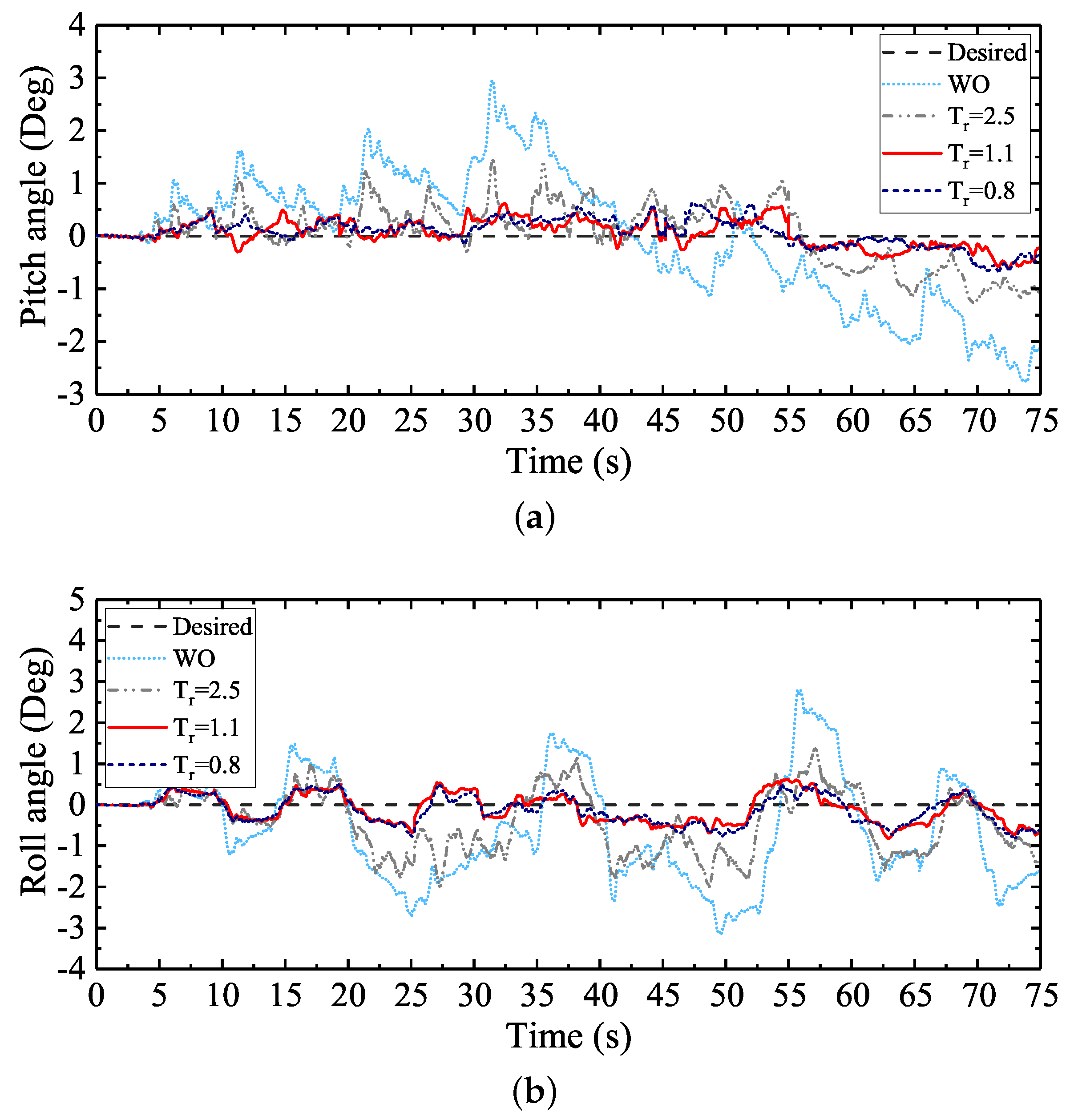
During hexapod locomotion, the body attitude trajectories are continually planned according to the motion state of the robot to keep the body balance. Therefore, the support leg trajectories of the robot are continuously updated to adjust the body deviations. Through this process, the body attitude trajectories during walking will be optimized and the walking balance of the robot will be ensured.

 ,
, 


