A Two-Stage Method for Target Searching in the Path Planning for Mobile Robots

Abstract
:1. Introduction
2. Problem Description
3. A Two-Stage Model for VCPP
3.1. Mathematical Model
3.2. A Two-Stage Model Design
4. Solving Methods
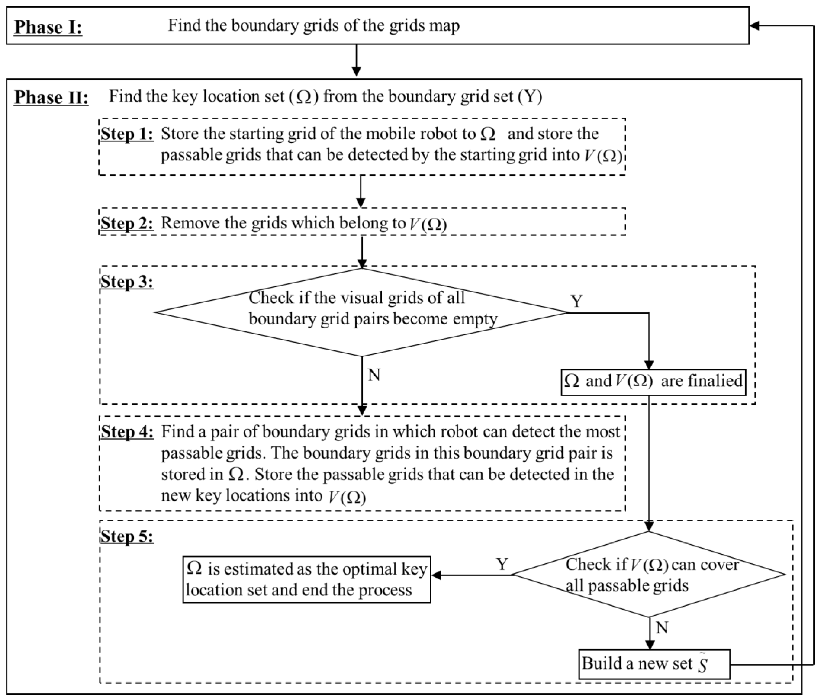
4.1. Stage I: A Heuristic Method
- Step 1: store the starting grid of the mobile robot to the key location set ; and store the passable grids that can be detected by the starting grid into the visible grid set of the key locations, i.e., .
- Step 2: remove the grids which belong to in the visual grids of all boundary grid pairs.
- Step 3: check if the visual grids of all boundary grid pairs become empty. If so, the key location set () and visible grid set are finalized, and go to Step 5. Otherwise, go to Step 4.
- Step 4: find a pair of boundary grids in which robot can detect the most passable grids. If there are multiple boundary grid pairs in which robot can detect the most passable grids, we select the boundary grid pair which is closest to the starting grid. The boundary grids in this boundary grid pair is stored in the key location set (). Store the passable grids that can be detected in the new key locations into the visible grid set of key locations (). Then, return to Step 2.
- Step 5: check if the visible grid set of key locations () can cover all passable grids. If so, the key location set () is estimated as the optimal key location set and end the process. If cannot cover all passable grids, we need to build a new set . The new set only retains these passable grids which cannot be detected in the original set S. Replace set S with set and add these passable grids in the original set S that already be detected to set O. Then, repeat the Phase I.
- (1)
- Set the starting grid 7 to the key location set ; and store the passable grids that can be detected ({7,8,12,13}) into the visible grid set of the key locations .
- (2)
- Remove the grids belonging to in the visual grids of boundary grid pairs .
- (3)
- If the visual grids of all boundary grid pairs are not empty, then go to next step.
- (4)
- Find some pair of boundary grids in which the robot can detect the most passable grids (i.e., {12,14}, {14,17}, {8,18}, {9,18}, {14,18}). Since {12,14} is the closest one, grids 12 and 14 are stored into the key location set (). Then the new key locations set is ({9,14,17,18,19}).
4.2. Stage II: Ant Colony Optimization Algorithm (ACO)
- Step 1: Initialization. Initialize the number of ants M, pheromone importance factor , pheromone concentrations , importance factor of heuristic function , volatile degree of pheromone , the total amount of pheromone released Q, the maximum number of iterations , and the initial number of iterations .
- Step 2: Construct the solution space. The ants are randomly placed at different starting locations. Each ant () determines the next location to visit based on the probability calculated by Equations (18) and (19) until all the ants have reached all locations .
- is the probability of ant transferring from location i to j at iteration t.
- is the pheromone concentration on the connection path between i and j at t.
- illustrates the distance of those key locations i and j.
- is the frequency of the robot which is unable to search for the target at the location j.
- is the set of locations to be visited for ant .
- is the pheromone importance factor. The larger , the more significant the role of pheromone concentration in the path selection.
- is the critical factor of heuristic function. The larger , the more significant the role of the heuristic function in the path selection. That is, ants will move to key locations with short distances with a high probability.
- Step 3: Determine the optimal solution. The path length of each ant will be calculated according to the distance between each key position, and all paths are recorded in the record table. Meanwhile, we record the optimal solution in the current number of iterations.
- Step 4: Update the pheromone. The pheromone concentration on the connection path between key locations is updated according to Equations (20)–(22).
- Step 5: Judge the termination conditions. If the maximum iteration is met, stop calculation and output the optimal result. Otherwise, iteration increases by one, the records of the ant paths are cleared and return to Step 2.
5. Evaluation
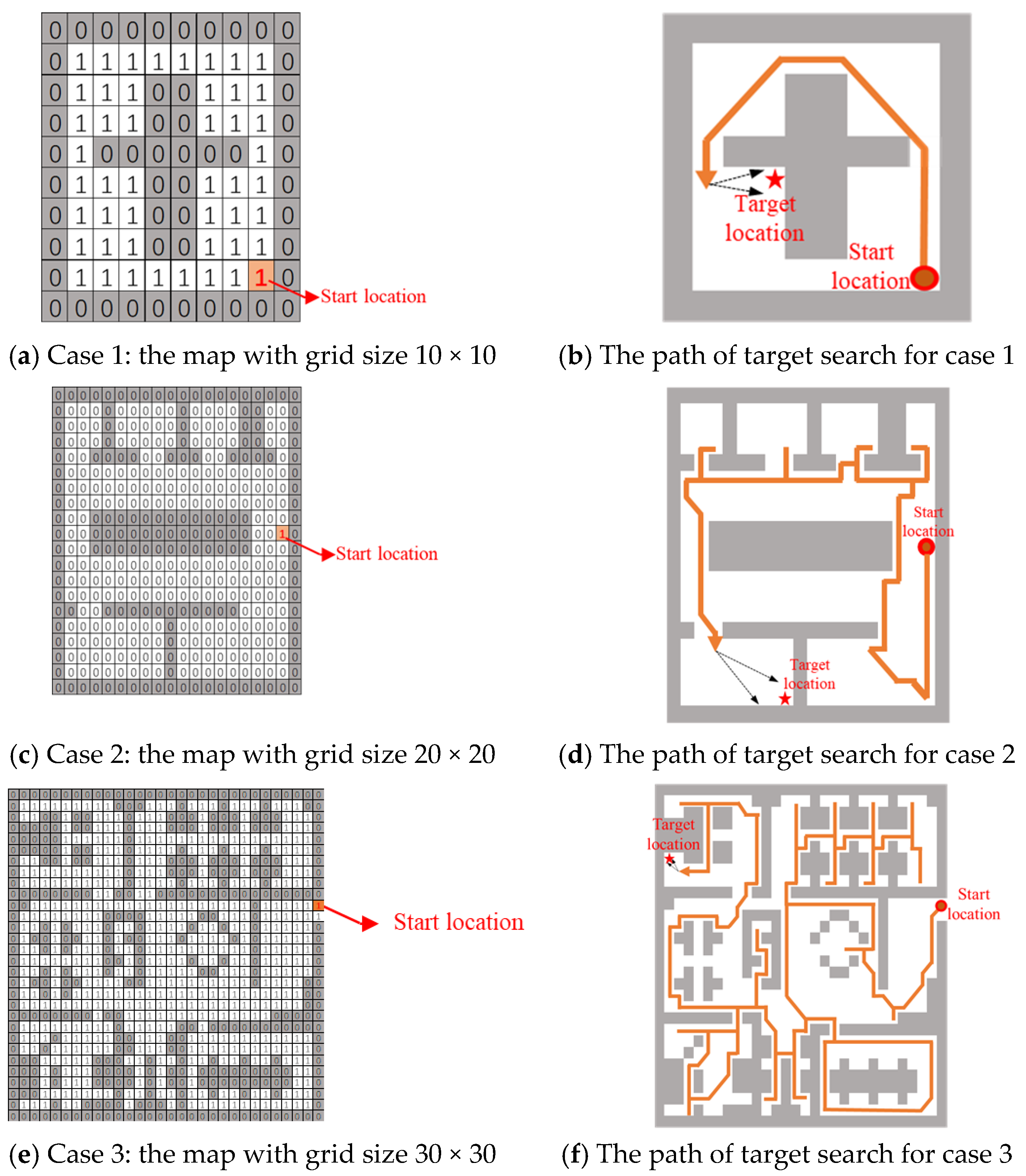
5.1. Case Scenarios
5.2. Result Comparisons with Two Other Algorithms
- (1)
- Rule-based Algorithm (RBA): Rule-based Algorithm is a heuristic algorithm, including the internal spiral coverage algorithm (ISC) for full coverage path planning of sweeping robot and the frontier-based algorithm for autonomous exploration of the robot, etc. The inner spiral coverage algorithm was initially proposed by Butler et al. [19] based on the contact sensor algorithm. The basic idea of the internal spiral coverage algorithm is that the mobile robot advances clockwise or counterclockwise to traverse the entire work environment. The frontier-based algorithm for autonomous exploration of the robot was proposed by Brian et al. [20]. Frontiers are regions on the boundary between unexplored and explored space. To gain the newest and useful information, the robot must move to the borders and explore again.
- (2)
- Genetic Algorithm (GA): GA is an intelligent algorithm that was proposed by Holland in 1975 [21]. It is noted that GA has a strong global search ability and is suitable for discrete variable optimization problems. It imitates biological inheritance and evolution and introduces the concept of survival of the fittest in evolution into the algorithm.
5.2.1. Average Target Search Time
5.2.2. Path Length of Vision Complete Coverage of Passable Area
5.3. Results with the Prior Knowledge of Target Frequency
5.4. Results of the Test in a Real Environment with a Real Robot
6. Conclusions
Author Contributions
Funding
Conflicts of Interest
References
- Lakshmanan, A.K.; Mohan, R.E.; Ramalingam, B.; Le, A.V.; Ilyas, M. Complete coverage path planning using reinforcement learning for tetromino based cleaning and maintenance robot. Autom. Constr. 2020, 112, 103078. [Google Scholar] [CrossRef]
- Yakoubi, A.M.; Laskri, M.T. The path planning of cleaner robot for coverage region using Genetic Algorithms. J. Innov. Digit. Ecosyst. 2016, 3, 37–43. [Google Scholar] [CrossRef] [Green Version]
- Wang, Z.; Li, H.; Zhang, X. Construction waste recycling robot for nails and screws: Computer vision technology and neural network approach. Autom. Constr. 2019, 97, 220–228. [Google Scholar] [CrossRef]
- Kim, J. Underwater surface scan utilizing an unmanned underwater vehicle with sampled range information. Ocean Eng. 2020, 207, 107345. [Google Scholar] [CrossRef]
- Sandamurthy, K.; Ramanujam, K. A hybrid weed optimized coverage path planning technique for autonomous harvesting in cashew orchards. Inf. Process. Agric. 2019, 7, 152–164. [Google Scholar] [CrossRef]
- Ellefsen, K.O.; Lepikson, H.A.; Albiez, J.C. Multiobjective coverage path planning: Enabling automated inspection of complex, real-world structures. Appl. Soft Comput. 2019, 61, 264–282. [Google Scholar] [CrossRef] [Green Version]
- Glorieux, E.; Franciosa, P.; Ceglarek, D. Coverage path planning with targetted viewpoint sampling for robotic free-form surface inspection. Robot. Comput. Integr. Manuf. 2020, 61, 101843.1–101843.11. [Google Scholar] [CrossRef]
- Galceran, E.; Carreras, M. Planning coverage paths on bathymetric maps for in-detail inspection of the ocean floor. In Proceedings of the 2013 IEEE International Conference on Robotics and Automation, Karlsruhe, Germany, 6–10 May 2013. [Google Scholar]
- Mansouri, S.S.; Kanellakis, C.; Georgoulas, G.; Kominiak, D.; Gustafsson, T.; Nikolakopoulos, G. 2D Visual Area Coverage and Path Planning Coupled with Camera Footprints. Control Eng. Pract. 2018, 75, 1–16. [Google Scholar] [CrossRef]
- Wang, P.; Krishnamurti, R.; Gupta, K. View Planning Problem with Combined View and Traveling Cost. In Proceedings of the 2017 IEEE International Conference on Robotics and Automation, Roma, Italy, 10–14 April 2007. [Google Scholar]
- An, W.; Shao, F.M.; Meng, H. The coverage-control optimization in sensor network subject to sensing area. Comput. Math. Appl. 2009, 57, 529–539. [Google Scholar] [CrossRef] [Green Version]
- Angella, F.; Reithler, L.; Gallesio, F. Optimal Development of Cameras for Video Surveillance Systems. In Proceedings of the IEEE International Conference on Advanced Video and Signal Based Surveillance (AVSS), London, UK, 5–7 September 2007; pp. 388–392. [Google Scholar]
- Arain, M.A.; Cirillo, M.; Bennetts, V.H.; Schaffernicht, E.; Lilienthal, A.J. Efficient Measurement Planning for Remote Gas Sensing with Mobile Robots. In Proceedings of the 2015 IEEE International Conference on Robotics and Automation, Seattle, WA, USA, 26–30 May 2015; pp. 3428–3434. [Google Scholar]
- Applegate, D.L. The Traveling Salesman Problem: A Computational Study; Princeton University Press: Princeton, NJ, USA, 2006. [Google Scholar]
- Hart, P.E.; Nilsson, N.J.; Raphael, B. A formal basis for the heuristic determination of minimum cost paths. IEEE Trans. Syst. Sci. Cybern. 1986, 4, 100–107. [Google Scholar] [CrossRef]
- Majeed, A.; Lee, S. A New Coverage Flight Path Planning Algorithm Based on Footprint Sweep Fitting for Unmanned Aerial Vehicle Navigation in Urban Environments. Appl. Sci. 2019, 9, 1470. [Google Scholar] [CrossRef] [Green Version]
- Rueda, R.; Ruiz, L.G.B.; Cuellar, M.P.; Pegalajar, M.C. An Ant Colony Optimization approach for symbolic regression using Straight Line Programs. Application to energy consumption modelling. Int. J. Approx. Reason. 2020, 121, 23–38. [Google Scholar] [CrossRef]
- Kumar, R.; Singh, R.; Ashfaq, H. Stability enhancement of multi-machine power systems using Ant colony optimization-based static Synchronous Compensator. Comput. Electr. Eng. 2020, 83, UNSP 106589. [Google Scholar] [CrossRef]
- Butler, Z.; Rizzi, A.; Hollis, R. Contact sensor-based coverage of coverage of rectilinear environments. In Proceedings of the IEEE International Symposium on Intelligent Control Intelligent Systems and Semiotics, Cambridge, MA, USA, 15–17 September 1999; pp. 266–271. [Google Scholar]
- Yamauchi, B. A frontier-based approach for autonomous exploration. In Proceedings of the 1997 IEEE International Symposium on Computational Intelligence in Robotics and Automation, Monterey, CA, USA, 10–11 July 1997. [Google Scholar]
- Holland, J.H. Adaptation in Natural and Artificial Systems: An Introductory Analysis with Applications to Biology, Control, and Artificial Intelligence; MIT Press: Cambridge, MA, USA, 1992. [Google Scholar]
- Tomioka, Y.; Takara, A.; Kitazawa, H. Generation of an Optimum Patrol Course for Mobile Surveillance Camera. IEEE Trans. Circuits Syst. Video Technol. 2012, 22, 216–224. [Google Scholar] [CrossRef]


| Parameters | |
|---|---|
| S | set of passable grids |
| P | optimal path |
| n | number of observation locations of P |
| i | the ID of the observation locations of P, |
| observation location, | |
| Z | set of subpath of P |
| a subpath which refers that robot moves from to , | |
| union of a series of visible grid sets detected by Z | |
| the moving cost associated with , | |
| g | the ID of the starting location of a mobile robot |
| Ω | set of key locations |
| a binary indicating if the grid k is set as a key location, | |
| set of passable grids that the robot can detect at key location k | |
| union of passable grids visible that the robot can detect at all key locations | |
| number of key locations in | |
| binary factor, which indicates whether the mobile robot moves from key location j to k, | |
| distance between key location j and k, | |
| probability of the robot unable to search for the target at the key location k, | |
| number of test times of the robot unable to search for the target at key location k, | |
| W | total number of test times |
| subset of set | |
| Path Length (m) | Increase Rate of Path Length (%) | Average Time (s) | Reduce Rate of Average Time (%) | |||
|---|---|---|---|---|---|---|
| OA | IOA | OA | IOA | |||
| Case 1 | 15 | 18 | 20 | 10.71 | 9.7 | 9.43 |
| Case 2 | 69 | 84 | 21.74 | 49.31 | 46.67 | 5.35 |
| Case 3 | 231 | 234 | 1.3 | 177.49 | 143.24 | 19.3 |
Publisher’s Note: MDPI stays neutral with regard to jurisdictional claims in published maps and institutional affiliations. |
© 2020 by the authors. Licensee MDPI, Basel, Switzerland. This article is an open access article distributed under the terms and conditions of the Creative Commons Attribution (CC BY) license (http://creativecommons.org/licenses/by/4.0/).
Share and Cite
Song, T.; Huo, X.; Wu, X. A Two-Stage Method for Target Searching in the Path Planning for Mobile Robots. Sensors 2020, 20, 6919. https://doi.org/10.3390/s20236919
Song T, Huo X, Wu X. A Two-Stage Method for Target Searching in the Path Planning for Mobile Robots. Sensors. 2020; 20(23):6919. https://doi.org/10.3390/s20236919
Chicago/Turabian StyleSong, Tao, Xiang Huo, and Xinkai Wu. 2020. "A Two-Stage Method for Target Searching in the Path Planning for Mobile Robots" Sensors 20, no. 23: 6919. https://doi.org/10.3390/s20236919