This section will discuss the feature extraction and machine learning methodology. The proposed work follows the supervised machine learning methodology. The steps involved in our proposed methodology are feature extraction, preprocessing, training, testing, and validation.
3.1. Feature Extraction
In the context of ML-based earthquake detection, amplitude and frequency are the two key pieces of information among different statistics of the accelerometer signal. Therefore, based on these two statistics, we extracted features from X, Y, and Z components in the time and frequency domains. Time domain features include features used in MyShake and our proposed features. The MyShake features are the following.
IQR (Interquartile Range): IQR is the interquartile range
–
of the 3 component vector sum
;
where
X,
Y, and
Z are the acceleration components.
(Cumulative Absolute Velocity):
feature is the cumulative measure of the
in the time window and is calculated as
where
s is the total time period of the feature window in seconds, and
t is the time. In this work, we used a two-second feature window.
(Zero-Crossing):
is the maximum zero-crossing rate of
X,
Y, and
Z component and the zero-crossing rate of component
X can be calculated as:
where
N is the total length of the signal
X and
is indicator function.
IQR and CAV are the amplitude features, while ZC is the frequency feature, and these are proposed in [
6,
30]. These features detect earthquakes and can discriminate non-earthquake data, but through exhaustive experimental evaluations and also its implementation in the static environment as given in our previous work, we found that in a noisy environment (noisy sensors or external events), its performance can be degraded. Moreover, a dynamic environment—in which the variety of human activities that include some challenging activities whose signal patterns are similar earthquake patterns—can also degrade the performance of the model trained on these features. We observed that among the three features, zero-crossing is more sensitive to noise and creates false alarms even if there is wavering involving only one component. This is due to the fact that it counts the feature value for each component and then selects the maximum one. Hence, if there is a count at only one component, then it will select that value and discard the zero-crossing information of the other two components. We observe that earthquake motion has a zero-crossing rate at more than one component simultaneously, while other data—particularly noise data—have zero-crossing rates at only one component most of the time, as given in
Table 2. Two-second feature window with a 1-second sliding window is used to count ZC in both earthquake data and noise data, where, for the earthquake data, we selected 3 s of the strongest portion of the earthquake. Further details about datasets are given in the results section.
This sensitivity issue not only affects the performance of the machine learning model in a dynamic environment (when the sensors are assumed to be smartphones used in daily life) but also affects the model performance while in a fixed-sensors environment. Therefore, to overcome this issue, we tested different variations and statistical features of the amplitude and frequency characteristics of the signal. After extensive experiments, we proposed some variants of the zero-crossings, which are the following.
Max ZC: Counts for that component whose maximum absolute amplitude value is greater than the other two components when there is more than one zero-crossings at a particular time t. Otherwise, it will behave like the ZC feature.
Min ZC: Counts for the minimum one, which has lowest absolute amplitude value among the three, if there are zero-crossings in more than one component.
Max Non ZC: This feature counts the maximum absolute amplitude component for non-zero-crossings when there is more than one non-zero-crossings simultaneously at a particular time.
These features are also based on the frequency and amplitude information of the signal; however, these are more specific and consider the other statistics, like multi-component zero-crossings and the frequency information, when there is no zero-crossing. The non-zero-crossing statistic is also important, because if the occurrences of ZC indicate the probability of an earthquake situation, then this feature indicates the probability of a normal situation. Similarly, the multi-component property of these features is also helpful to discriminate human activities from earthquake samples more efficiently.
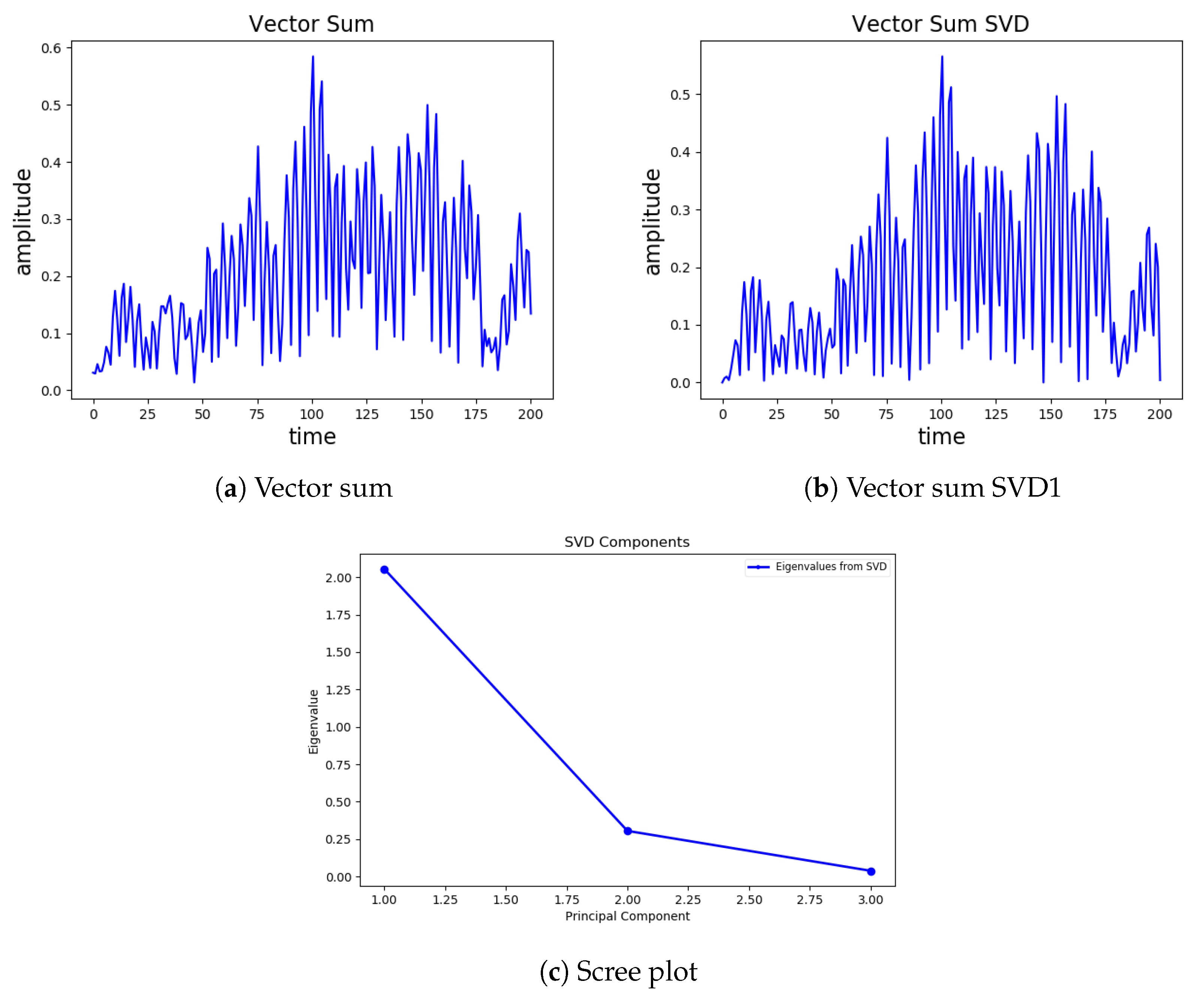
Apart from the proposed features, we also tested features from the frequency domain, i.e., FFT (Fast Fourier Transform) [
31]. In order to consider only one component of FFT, we used a Singular Value Decomposition (SVD) method to decompose multi-dimensional data into one dimension [
32]. The SVD of an accelerometer matrix
A of three components, X, Y, and Z.
where,
A is an M x N matrix, where M represents two-second points, i.e., 200, and N is 3. SVD provides three new vectors
, which, if linearly combined, give back the approximated original vector; where
U is the set of singular vectors with singular values in vector
S,
is the primary direction. The new vectors are ordered, and the first vector explains most of the original acceleration amplitude and frequency information, as shown in
Figure 3.
Figure 3a depict almost the same structure; therefore, we select the first vector as a primary vector
from the given SVD’s, along with the first value
of
S, which is a scaling factor (give amplitude information of the given vector). We extracted the following three additional features.
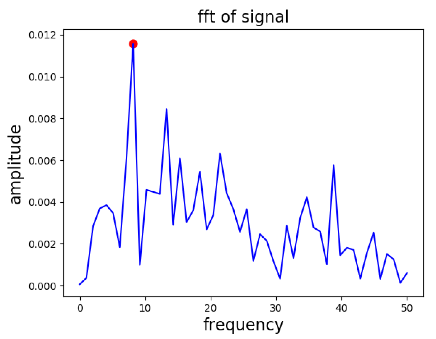
FFT: FFT of the given vector
is calculated, and we selected the frequency bin as a frequency feature that has the peak amplitude, as shown in
Figure 4.
SVD_Scale: The is considered the average amplitude feature.
SVD_ZC: We also computed the zero-crossing rate of the primary vector i.e., .
We also analyzed the tsfresh [
33], a time series feature-extraction python package for searching the computationally low and effective features such as c3, cid-ce, entropy, mean, and count-above-mean, etc. However, the feature space visualization was not more promising than the abovementioned features. Therefore, we selected only the above features for model training and testing.
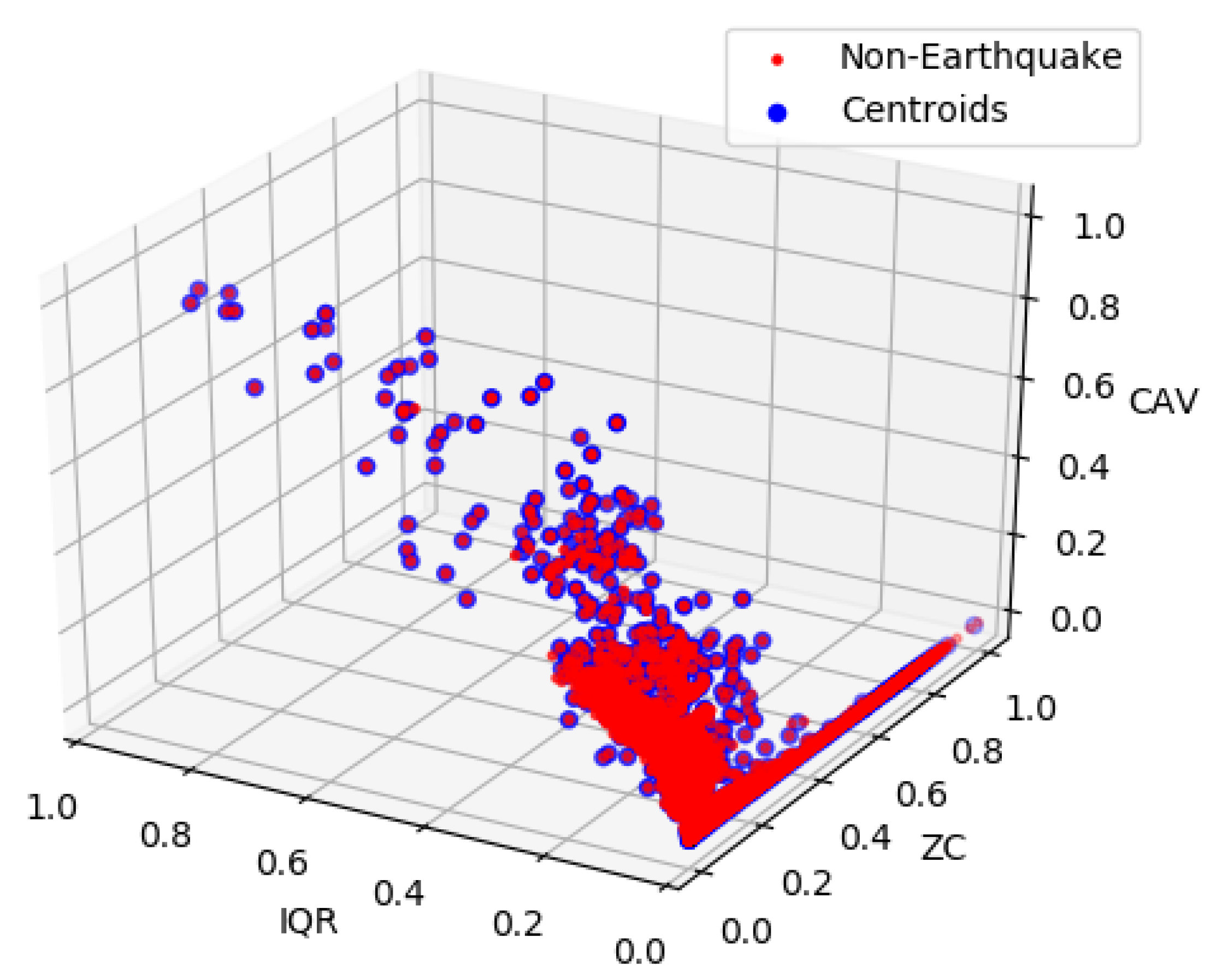
3.2. Pre-Processing
In our methodology, the pre-processing involved balancing the dataset and scaling the features to range from 0 to 1. Balancing is required because the imbalanced datasets greatly affect the performance of the machine learning model [
34]. In our case, the non-earthquake dataset (noise and human activities) is much larger than the earthquake dataset. Hence, we used the K-mean clustering algorithm to balance the non-earthquake dataset [
35]. Using the K-Mean, clusters of the non-earthquake data are created according to the total number of earthquake data points, and we used centroids of the clusters to represent the non-earthquake data. As shown in
Figure 5, centroids represent the original data points in the IQR, ZC, and CAV feature space.
Moreover, to improve the prediction performance and decrease the training time of the model, we also scaled data point
d to the range of 0 to 1 using the min-max scaler as follows:
3.3. Machine Learning Model
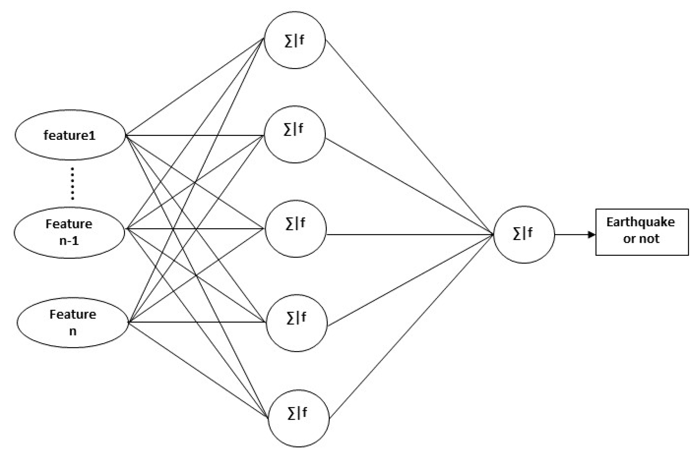
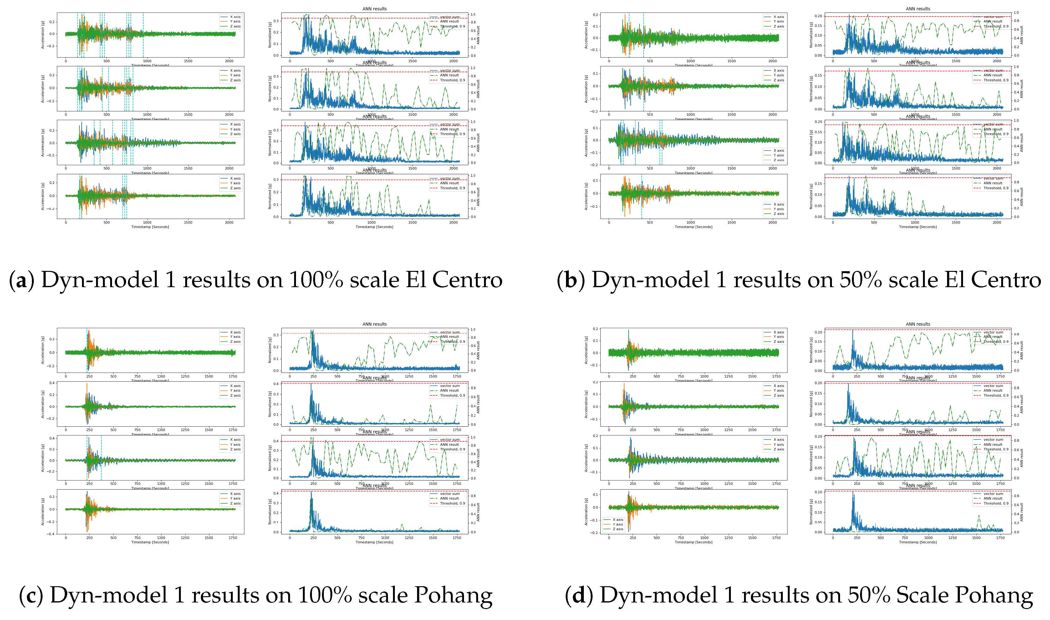
The ANN (Artificial Neural Network) algorithm is designed to accomplish the detection task using both the existing and proposed features [
12]. We used an X, 5, 1 layer network architecture for the training and testing of the ANN algorithm, as shown in
Figure 6, where X is the number of features input to the model. We kept the same five nodes of the hidden layer as proposed in [
6], because the number of features input to the model is 3, 4, or 5, and through experimental results, the 5-node hidden layer is still good for the given number of features. For training the models, we used a multi-layer perceptron (MLP) with the stochastic gradient descent solver [
36,
37,
38]. For the hidden layer and output layer, the inputs from the previous layer to each node will be first summed and then fed into an activation function as follows:
Here,
w denotes the weights vector,
d is the input vector,
b is the bias,
y is the output of the given node, and
is the non-linear activation function. The logistic sigmoid function is used as the activation function for hidden and output layers, which is defined on input
d as


