Figure 1.
Example of exudates, microaneurysms and hemorrhages in fundus images.
Figure 1.
Example of exudates, microaneurysms and hemorrhages in fundus images.
Figure 2.
Illustration of the local analysis in fundus images: (a) Visual representation of how the sliding window of dimensions loops a fundus image and (b) the resulting image grid composed by the centers of the sliding window in each position. This process is equivalent to a dense sampling. For the representation and (,) = () were used.
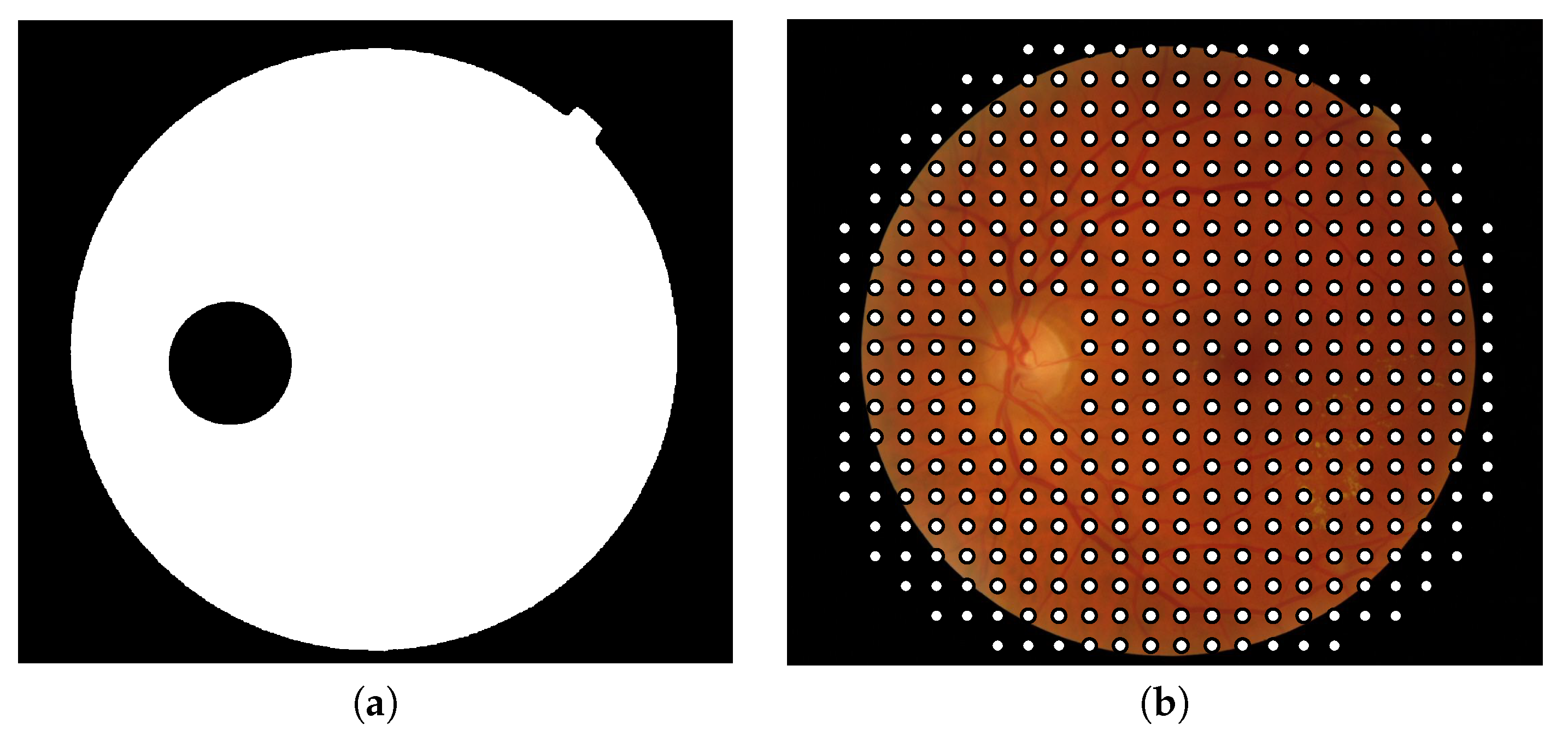
Figure 3.
(a) Binary mask used to exclude the patches containing optic disk pixels and the patches located out of the field of view and (b) center of the patches composing the final grid in which image descriptors will be applied.
Figure 3.
(a) Binary mask used to exclude the patches containing optic disk pixels and the patches located out of the field of view and (b) center of the patches composing the final grid in which image descriptors will be applied.
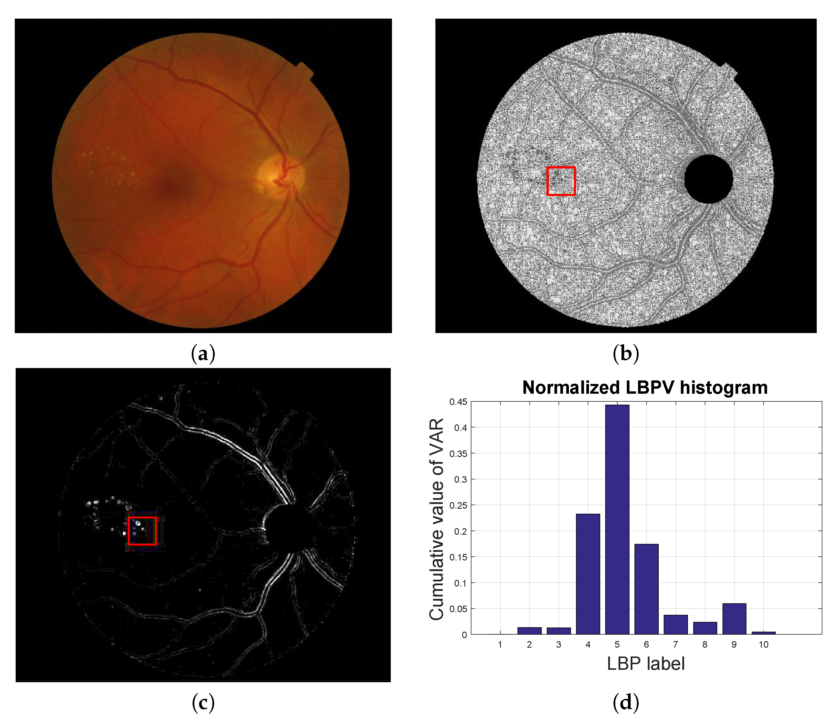
Figure 4.
Local texture analysis. (a) Original fundus image, (b) LBP image and (c) VAR image with a patch highlighted in red and (d) the LBPV normalized histogram computed for the red patch.
Figure 4.
Local texture analysis. (a) Original fundus image, (b) LBP image and (c) VAR image with a patch highlighted in red and (d) the LBPV normalized histogram computed for the red patch.
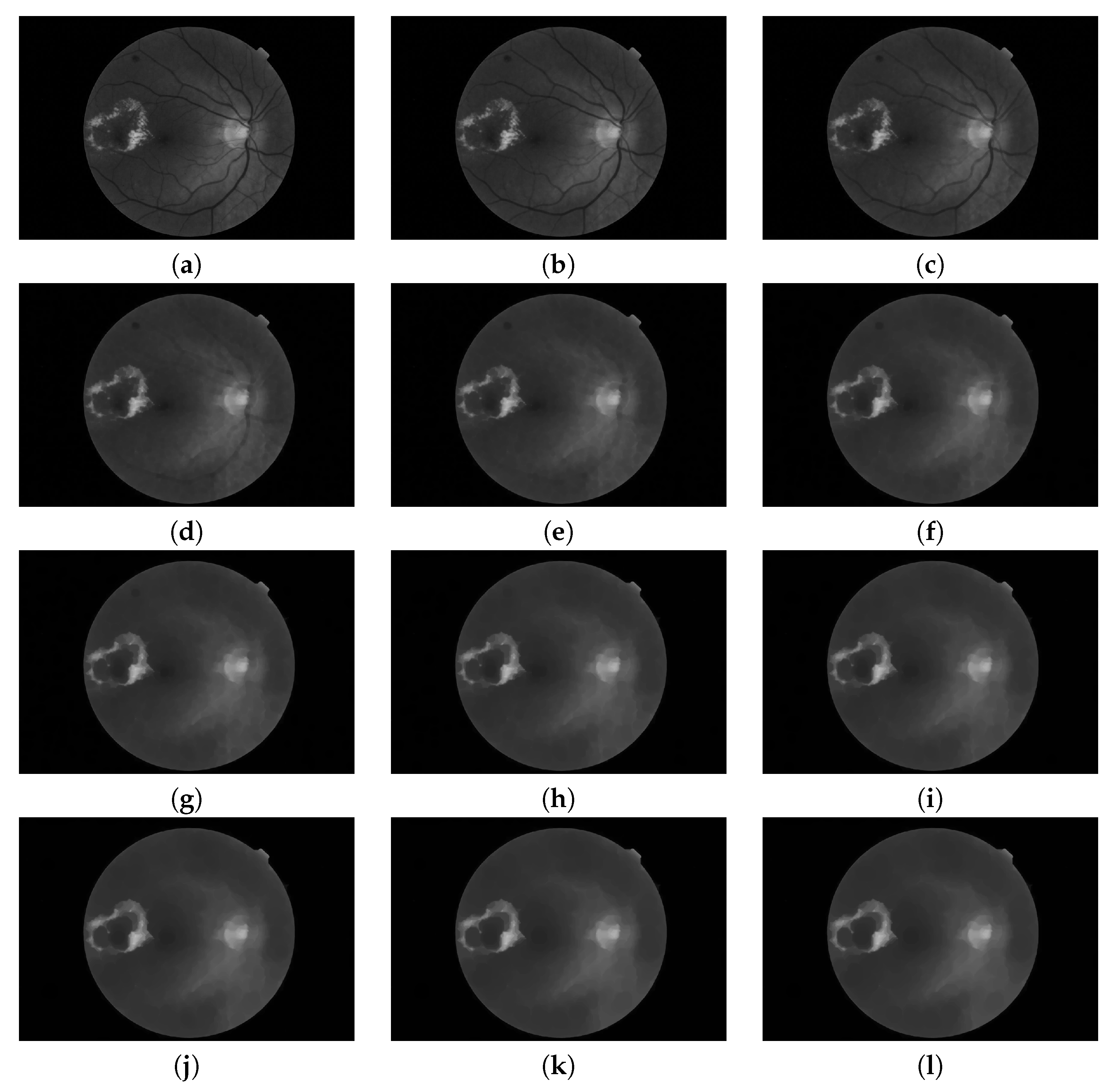
Figure 5.
Pyramid of openings computed for a fundus image using an isotropic structuring element. It is composed by 12 images (). (a) Original image; i.e., is the identity mapping; (b–k) are the results of applying the opening operator with increasing size (according to ) and (l) is the last image of the pyramid corresponding to the operation .
Figure 6.
Pyramid of closings computed from a fundus image using an isotropic structuring element. It is composed by 12 images (). (a) Original image; i.e., is the identity mapping; (b–k) are the results of applying the closing operator with increasing size (according to ) and (l) is the last image of the pyramid corresponding to the operation .
Figure 7.
(a,c) represent the local extraction of the granulometry and anti-granulometry curves from the morphological pyramids and . (b,d) show the pattern spectrum computed for the patch marked in red in each case.
Figure 7.
(a,c) represent the local extraction of the granulometry and anti-granulometry curves from the morphological pyramids and . (b,d) show the pattern spectrum computed for the patch marked in red in each case.
Figure 8.
A global pattern spectrum extracted by the combination of the granulometric and anti-granulometric profiles.
Figure 8.
A global pattern spectrum extracted by the combination of the granulometric and anti-granulometric profiles.
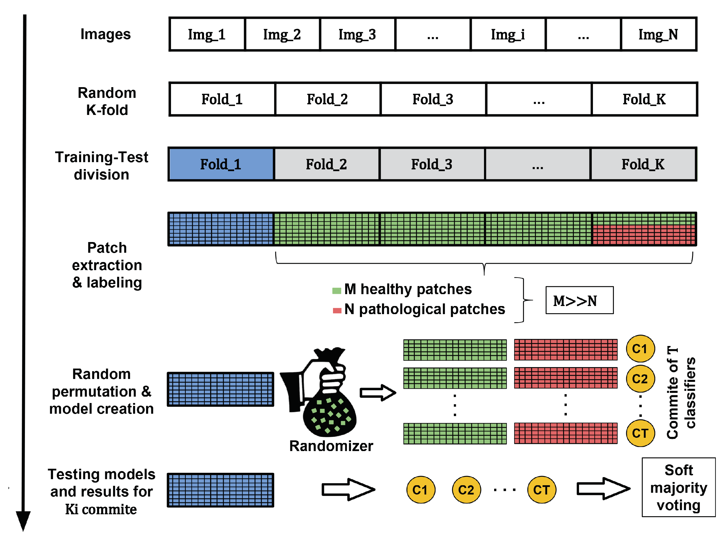
Figure 9.
Process of creating the machine learning models using a generic dataset. Green and red samples are used in the creation of the model while blue instances refer to the samples used in the testing stage.
Figure 9.
Process of creating the machine learning models using a generic dataset. Green and red samples are used in the creation of the model while blue instances refer to the samples used in the testing stage.
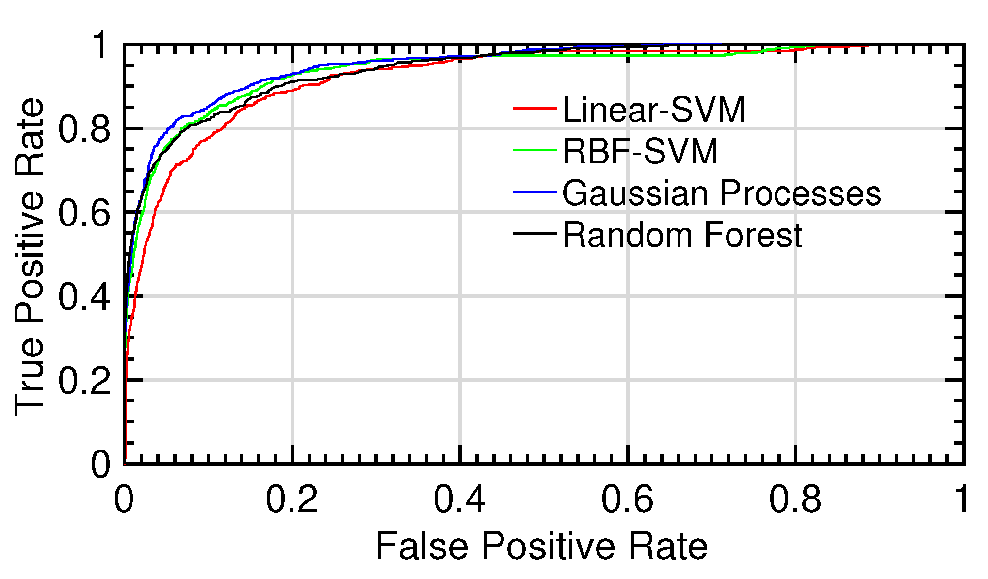
Figure 10.
ROC curves for the different tests.ROC curves for the different tests
Figure 10.
ROC curves for the different tests.ROC curves for the different tests
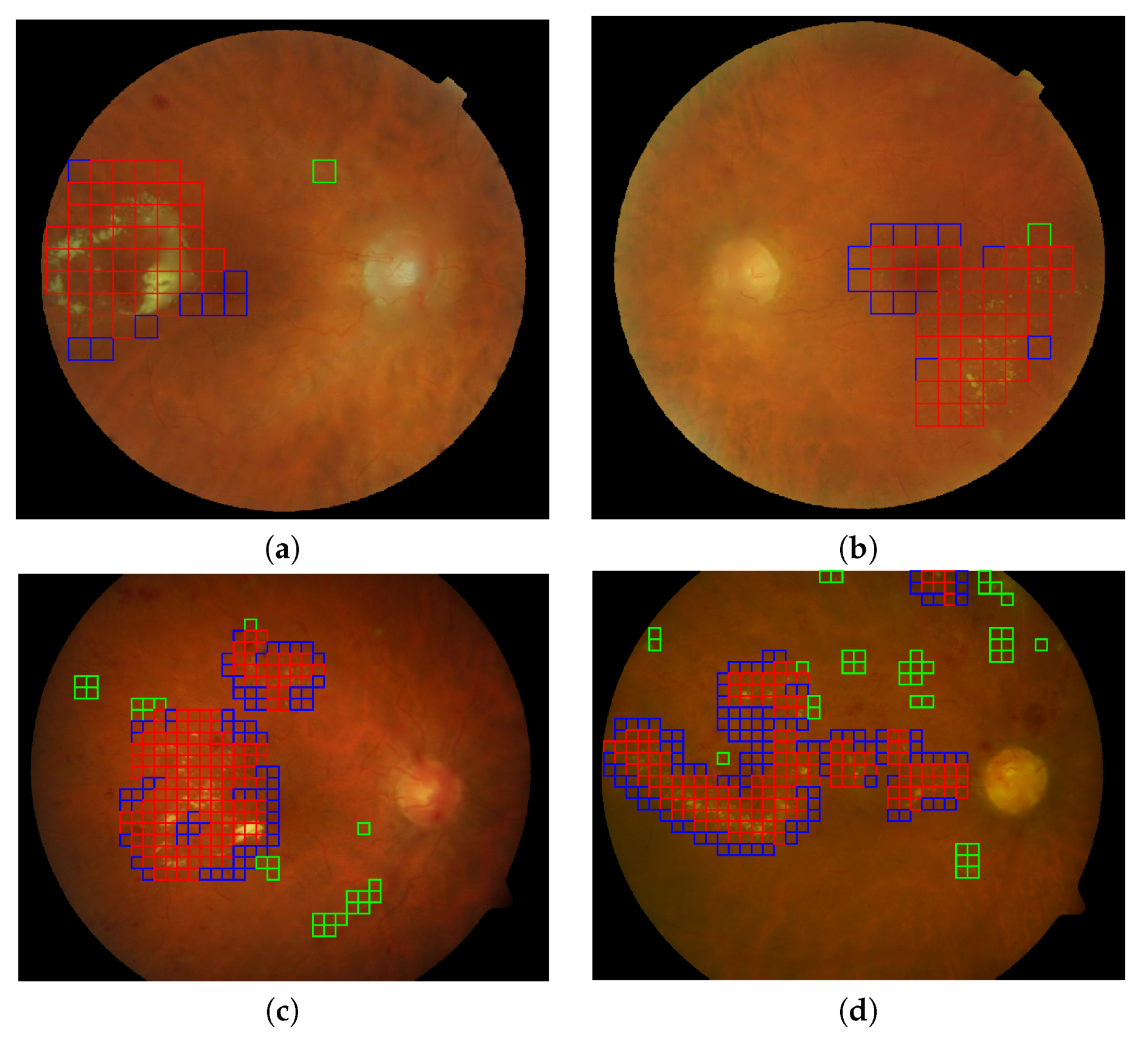
Figure 11.
Automatic lesion detection in four retinal images using the best configuration of feature vector and gaussian processes for classification. (a,b) Two representative images (DS000U30.jpg and DS0009NU.jpg) from the E-OPHTHA exudates database and (c,d) two representative image (image014.png and image016.png) from DIARETDB1 database. Red squares indicate the true positives, green squares the false positives and the blue squares reveal the false negative detections.
Table 1.
AUC, accuracy, sensitivity and specificity related to the exudate detection for E-OPHTHA exudates database taking into account different morphological input vectors to the SVM classifier.
Table 1.
AUC, accuracy, sensitivity and specificity related to the exudate detection for E-OPHTHA exudates database taking into account different morphological input vectors to the SVM classifier.
| | Accuracy | Sensitivity | Specificity | AUC |
|---|
| 0.6405 ± 0.0572 | 0.6137 ± 0.1378 | 0.6489 ± 0.0813 | 0.6701 ± 0.0617 |
| 0.6684 ± 0.0353 | 0.6009 ± 0.1449 | 0.6759 ± 0.0521 | 0.6907 ± 0.0601 |
| 0.7014 ± 0.0247 | 0.6396 ± 0.1420 | 0.7090 ± 0.0426 | 0.7337 ± 0.0777 |
| 0.5794 ± 0.0588 | 0.5105 ± 0.0887 | 0.5914 ± 0.0823 | 0.5783 ± 0.0366 |
| 0.7554 ± 0.0161 | 0.6592 ± 0.1179 | 0.7698 ± 0.0292 | 0.7877 ± 0.0524 |
| 0.6550 ± 0.0528 | 0.6223 ± 0.1243 | 0.6636 ± 0.0745 | 0.6946 ± 0.0546 |
| 0.7321 ± 0.0208 | 0.6394 ± 0.0839 | 0.7465 ± 0.0271 | 0.7543 ± 0.0461 |
| 0.7112 ± 0.0262 | 0.6446 ± 0.1344 | 0.7194 ± 0.0451 | 0.7482 ± 0.0684 |
| 0.6685 ± 0.0320 | 0.5935 ± 0.1363 | 0.6774 ± 0.0499 | 0.6882 ± 0.0564 |
| 0.7014 ± 0.0256 | 0.6346 ± 0.1376 | 0.7099 ± 0.0432 | 0.7349 ± 0.0749 |
| 0.7620 ± 0.0165 | 0.6648 ± 0.1124 | 0.7762 ± 0.0300 | 0.7924 ± 0.0493 |
Table 2.
AUC, accuracy, sensitivity and specificity related to the exudate detection for E-OPHTHA exudates database taking into account different input vectors to the SVM classifier. In particular, they are composed by texture and shape descriptors.
Table 2.
AUC, accuracy, sensitivity and specificity related to the exudate detection for E-OPHTHA exudates database taking into account different input vectors to the SVM classifier. In particular, they are composed by texture and shape descriptors.
| | Accuracy | Sensitivity | Specificity | AUC |
|---|
| LBPV | 0.8205 ± 0.0320 | 0.7389 ± 0.1034 | 0.8331 ± 0.0534 | 0.8684 ± 0.0435 |
| LBPV- | 0.8369 ± 0.0336 | 0.7603 ± 0.0897 | 0.8481 ± 0.0519 | 0.8834 ± 0.0397 |
| LBPV- | 0.8445 ± 0.0276 | 0.7657 ± 0.0894 | 0.8561 ± 0.0449 | 0.8872 ± 0.0384 |
| LBPV- | 0.8447 ± 0.0228 | 0.7496 ± 0.1079 | 0.8591 ± 0.0432 | 0.8803 ± 0.0409 |
| LBPV- | 0.8533 ± 0.0245 | 0.7721 ± 0.0857 | 0.8651 ± 0.0399 | 0.8948 ± 0.0351 |
Table 3.
AUC, accuracy, sensitivity and specificity related to the bright-lesion detection on E-OPHTHA exudates database for each classification method using a decision threshold .
Table 3.
AUC, accuracy, sensitivity and specificity related to the bright-lesion detection on E-OPHTHA exudates database for each classification method using a decision threshold .
| | Accuracy | Sensitivity | Specificity | AUC |
|---|
| Random Forests | 0.9508 ± 0.0084 | 0.4785 ± 0.1015 | 0.9921 ± 0.0043 | 0.9256 ± 0.0173 |
| Linear-SVM | 0.8533 ± 0.0245 | 0.7721 ± 0.0857 | 0.8651 ± 0.0399 | 0.8948 ± 0.0351 |
| RBF-SVM | 0.8796 ± 0.0229 | 0.8118 ± 0.0618 | 0.8851 ± 0.0296 | 0.9240 ± 0.0161 |
| Gaussian Processes | 0.8762 ± 0.0206 | 0.8348 ± 0.0650 | 0.8795 ± 0.0266 | 0.9353 ± 0.0174 |
Table 4.
AUC, accuracy, sensitivity and specificity related to the bright-lesion detection on E-OPHTHA exudates database. Results were optimized to the best sensitivity/specificity trade-off.
Table 4.
AUC, accuracy, sensitivity and specificity related to the bright-lesion detection on E-OPHTHA exudates database. Results were optimized to the best sensitivity/specificity trade-off.
| | Accuracy | Sensitivity | Specificity | |
|---|
| Random Forests | 0.8410 ± 0.0181 | 0.8418 ± 0.0178 | 0.8411 ± 0.0181 | 0.8999 ± 0.0214 |
| Linear-SVM | 0.8242 ± 0.0279 | 0.8243 ± 0.0284 | 0.8242 ± 0.0278 | 0.5771 ± 0.0958 |
| RBF-SVM | 0.8529 ± 0.0190 | 0.8531 ± 0.0193 | 0.8529 ± 0.0190 | 0.5835 ± 0.1012 |
| Gaussian Processes | 0.8581 ± 0.0221 | 0.8579 ± 0.0221 | 0.8579 ± 0.0222 | 0.5348 ± 0.0747 |
Table 5.
AUC, accuracy, sensitivity and specificity related to the bright-lesion detection on DIARETDB1 database for each classification method using a decision threshold .
Table 5.
AUC, accuracy, sensitivity and specificity related to the bright-lesion detection on DIARETDB1 database for each classification method using a decision threshold .
| | Accuracy | Sensitivity | Specificity | AUC |
|---|
| Random Forests | 0.9370 ± 0.0155 | 0.5096 ± 0.0478 | 0.9889 ± 0.0056 | 0.8852 ± 0.0314 |
| Linear-SVM | 0.8702 ± 0.0217 | 0.7396 ± 0.0528 | 0.8849 ± 0.0260 | 0.8879 ± 0.0301 |
| RBF-SVM | 0.8834 ± 0.0311 | 0.0.7509 ± 0.0489 | 0.8903 ± 0.0211 | 0.8901 ± 0.291 |
| Gaussian Processes | 0.8703 ± 0.0189 | 0.7705 ± 0.0500 | 0.8814 ± 0.0224 | 0.8971 ± 0.0286 |
Table 6.
AUC, accuracy, sensitivity and specificity related to the bright-lesion detection on DIARETDB1 database. Results were optimized to the best sensitivity-specificity trade-off.
Table 6.
AUC, accuracy, sensitivity and specificity related to the bright-lesion detection on DIARETDB1 database. Results were optimized to the best sensitivity-specificity trade-off.
| | Accuracy | Sensitivity | Specificity | |
|---|
| Random Forests | 0.8037 ± 0.0319 | 0.8027 ± 0.0324 | 0.8038 ± 0.0319 | 0.9006 ± 0.0146 |
| Linear-SVM | 0.8112 ± 0.0316 | 0.8107 ± 0.0315 | 0.8112 ± 0.0316 | 0.6207 ± 0.0440 |
| RBF-SVM | 0.8166 ± 0.0322 | 0.8154 ± 0.0321 | 0.8155 ± 0.0322 | 0.6334 ± 0.0401 |
| Gaussian Processes | 0.8184 ± 0.0324 | 0.8183 ± 0.0324 | 0.8184 ± 0.0324 | 0.6023 ± 0.0518 |
Table 7.
Comparison of exudate detection methods for the 47 retinal images with exudates of DIARETDB1 database.
Table 7.
Comparison of exudate detection methods for the 47 retinal images with exudates of DIARETDB1 database.
| Methods | Sensitivity | Specificity | PPV |
|---|
| Sopharak et al. [21] | 0.8482 | 0.9931 | 0.2548 |
| Walter et al. [16] | 0.6600 | 0.9864 | 0.1945 |
| Welfer et al. [17] | 0.7048 | 0.9884 | 0.2132 |
| Ghafourian and Pourreza [18] | 0.7828 | - | - |
| Proposed method | 0.8184 ± 0.0324 | 0.8183 ± 0.0324 | 0.4373 ± 0.1374 |
Table 8.
AUC, accuracy, sensitivity and specificity related to the dark-lesion detection (microaneurysms and hemorrhages) on DIARETDB1 database for each classification method studied in this work using a decision threshold .
Table 8.
AUC, accuracy, sensitivity and specificity related to the dark-lesion detection (microaneurysms and hemorrhages) on DIARETDB1 database for each classification method studied in this work using a decision threshold .
| | Accuracy | Sensitivity | Specificity | AUC |
|---|
| Random Forests | 0.9016 ± 0.0311 | 0.1718 ± 0.0800 | 0.9818 ± 0.0035 | 0.8150 ± 0.0356 |
| Linear-SVM | 0.7404 ± 0.0134 | 0.6969 ± 0.0865 | 0.7462 ± 0.0245 | 0.7975 ± 0.0367 |
| RBF-SVM | 0.7603 ± 0.0223 | 0.7299 ± 0.0821 | 0.7576 ± 0.0311 | 0.8209 ± 0.344 |
| Gaussian Processes | 0.7612 ± 0.0244 | 0.7489 ± 0.0844 | 0.7630 ± 0.0350 | 0.8344 ± 0.0330 |
Table 9.
AUC, accuracy, sensitivity and specificity related to the dark-lesion detection (microaneurysms and hemorrhages) on DIARETDB1 database. Results were optimized to the best sensitivity-specificity trade-off.
Table 9.
AUC, accuracy, sensitivity and specificity related to the dark-lesion detection (microaneurysms and hemorrhages) on DIARETDB1 database. Results were optimized to the best sensitivity-specificity trade-off.
| | Accuracy | Sensitivity | Specificity | |
|---|
| Random Forests | 0.7397 ± 0.0328 | 0.7391 ± 0.0320 | 0.7398 ± 0.0329 | 0.8645 ± 0.0329 |
| Linear-SVM | 0.7262 ± 0.0329 | 0.7261 ± 0.0324 | 0.7262 ± 0.0330 | 0.5170 ± 0.0591 |
| RBF-SVM | 0.7498 ± 0.0277 | 0.7375 ± 0.0301 | 0.7374 ± 0.0302 | 0.5554 ± 0.0601 |
| Gaussian Processes | 0.7562 ± 0.0290 | 0.7561 ± 0.0289 | 0.7562 ± 0.0290 | 0.5036 ± 0.0712 |
Table 10.
Comparison of dark-lesion detection methods for the 45 retinal images with microaneurysms or hemorrhages of DIARETDB1 database.
Table 10.
Comparison of dark-lesion detection methods for the 45 retinal images with microaneurysms or hemorrhages of DIARETDB1 database.
| Methods | Sensitivity | Specificity | AUC |
|---|
| Rocha et al. [54] | 0.9000 | 0.6000 | 0.7640 |
| Roychowdhury et al. [55] | 0.7550 | 0.9373 | 0.8263 |
| Ashraf et al. [56] | 0.6763 | 0.6278 | 0.6500 |
| Junior and Welfer [57] | 0.8769 | 0.9244 | - |
| Proposed method | 0.7561 ± 0.0301 | 0.7562 ± 0.0290 | 0.8344 ± 0.0330 |


