Experiment of Structural Geometric Morphology Monitoring for Bridges Using Holographic Visual Sensor


Abstract
:1. Introduction
2. Theoretical Fundamentals
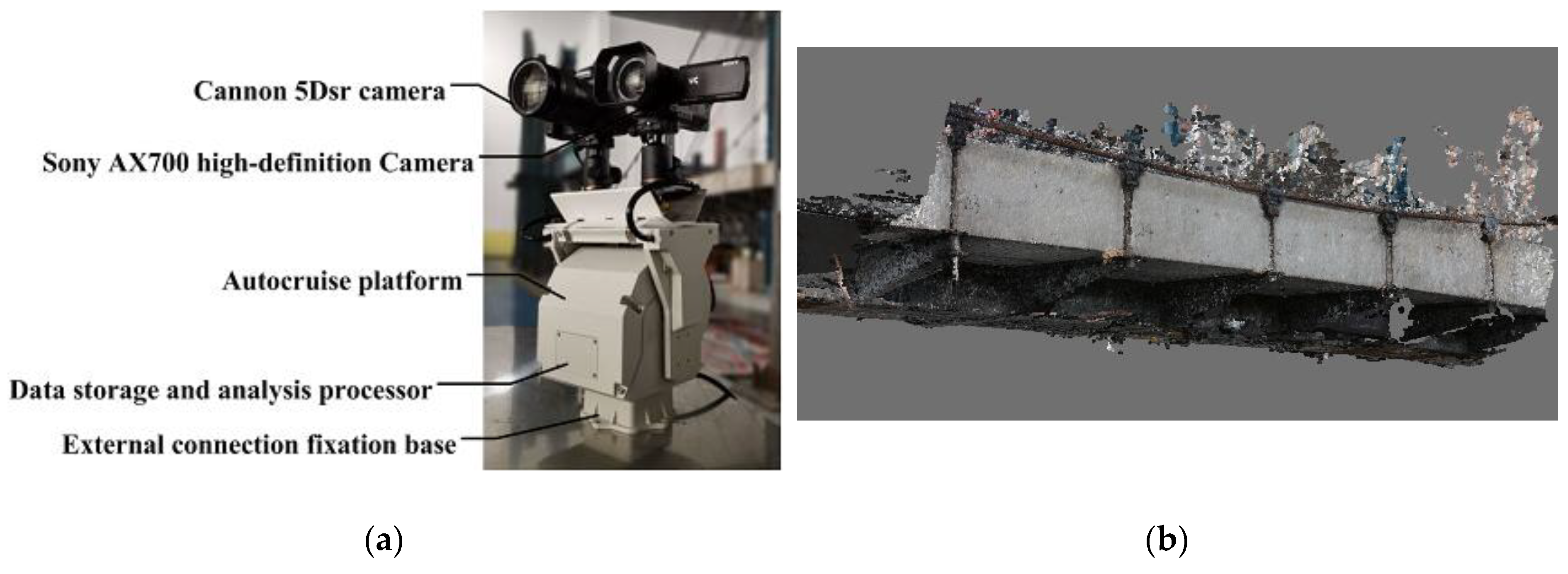
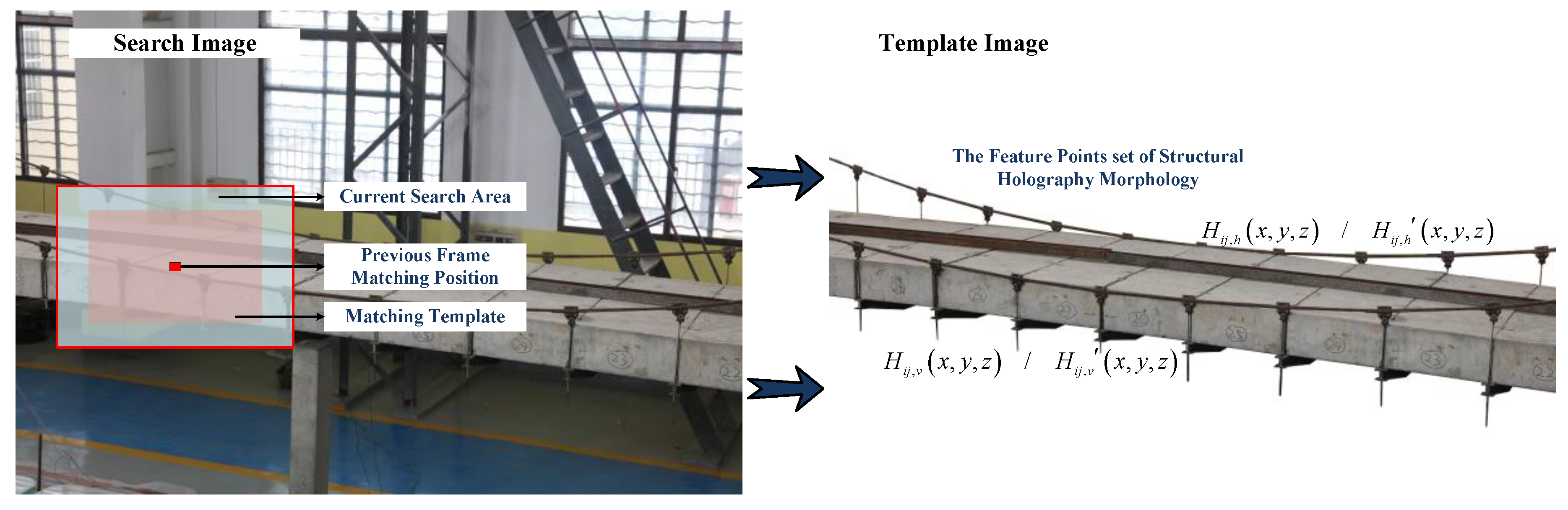
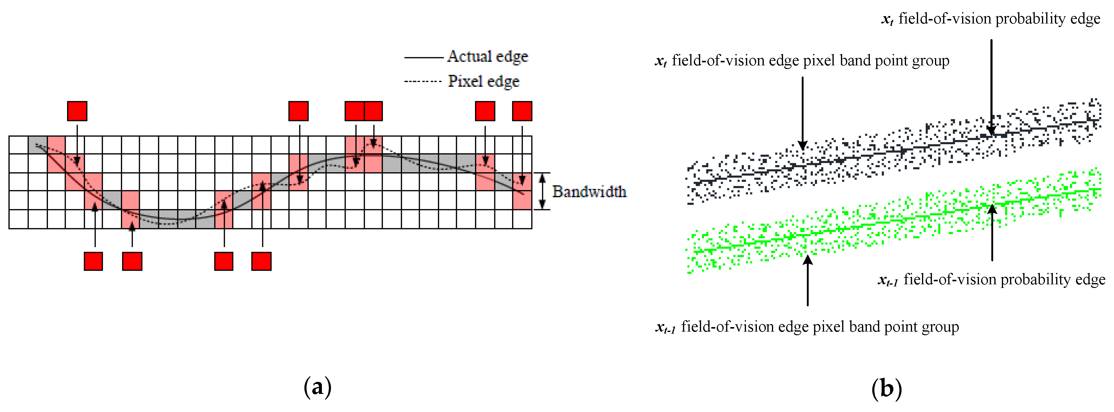
2.1. Holographic Visual Sensor
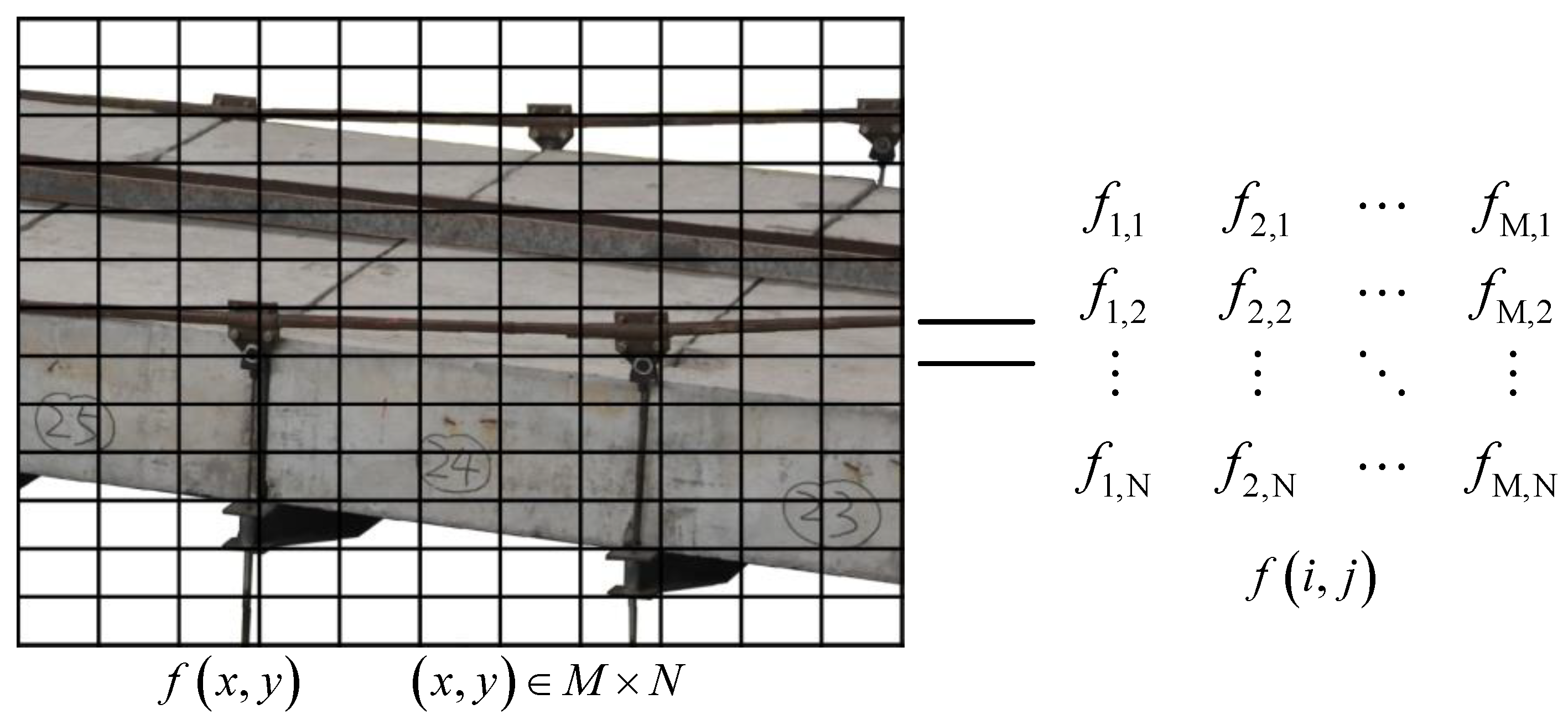
2.2. The Spatial and Temporal Series Data
3. Experimental Study
3.1. Experimental Setup and Procedure
3.2. Holographic Visual Sensor Based Characterization Parameters of Morphology Results
3.3. Structural Geometry Monitoring Analysis Using the Spatial and Temporal Series Data
4. Conclusions
- (1)
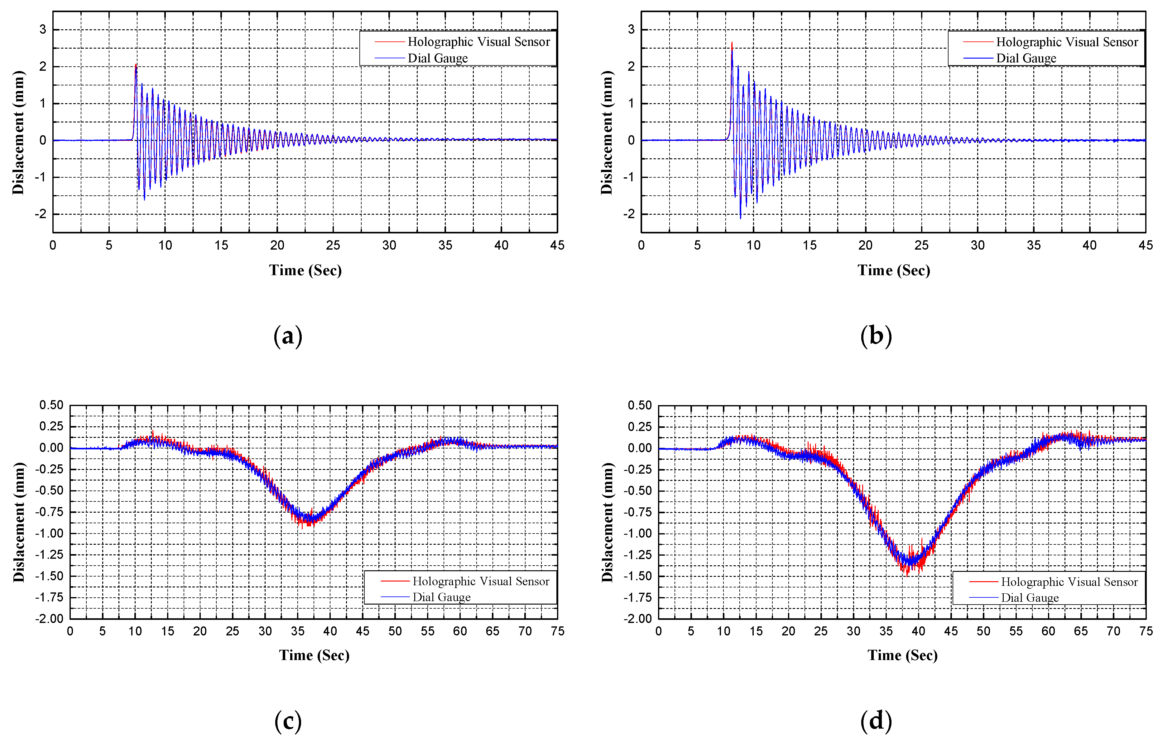
- Laboratory experiments on 24 m-span self-anchored suspension bridge demonstrate that holographic full-field displacement and vibration signal can be accurately, sensitively and simultaneously measured in multi-damage/operating conditions using holographic visual sensor, and the identified full-field displacements and natural frequencies by the holographic visual sensor match well with those by using dial gauges and accelerometers.
- (2)
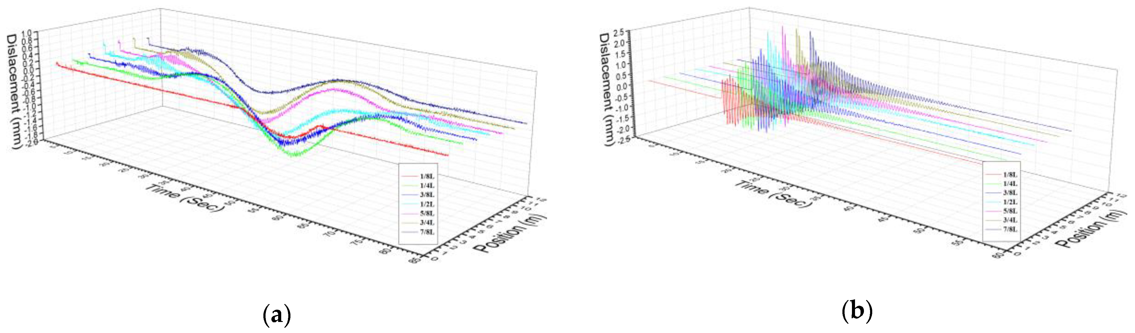
- The holographic visual sensor can arrange dense and continuous pixel-level/subpixel-level virtual measuring points on the surface of the tested object space, and the denser full-field displacement and smoother mode shapes can be further extracted, which makes it possible to dynamically update a model of digital twins, structural condition assessment, and intelligent damage identification methods.
- (3)
- As raised in this study, a holographic visual sensor is utilized to monitor holography geometric morphology of the bridge structure dependent on series data of structural holography images. In terms of normal deformations free of damages and abnormal deformations with damages, holography geometric morphology monitoring shows a strong capability in identifying their features, and accurately reflecting the real change in structural properties under various damage/action conditions.
- (4)
- It is much more likely for the test results here to suffer the influence of system noise interference and dramatic ambient light changes. Moreover, different illumination intensities cause certain structural response signal differences and losses. Concerned with environmental interference and noise influence, a microscopic theory and noise reduction anti-disturbance autoencoders (i.e., denoising AE (DAE) and contractive AE (CAE)) are recommended in this study, with the goal of lowering relevant errors and improving holographic visual sensor accuracy and algorithm stability. Once actions of noise and illuminance, etc., are further eliminated, not only can the integrity of response signals be effectively improved, but more abundant structural performance information can be retained.
Author Contributions
Funding
Acknowledgments
Conflicts of Interest
References
- Feng, D.M.; Feng, M.Q. Computer Vision for SHM of Civil Infrastructure: From Dynamic Response Measurement to Damage Detection—A review. Eng. Sturct. 2018, 156, 105–117. [Google Scholar] [CrossRef]
- Editorial Department of China Journal of Highway and Transport. Review on China’s Bridge Engineering Research: 2014. China J. Highw. Transp. 2014, 27, 1–96. [Google Scholar]
- Sun, L.M.; Shang, Z.Q.; Xia, Y. Development and Prospect of Bridge Structural Health Monitoring in the Context of Big Data. China J. Highw. Transp. 2019, 32, 1–20. [Google Scholar]
- Ye, X.W.; Dong, C.Z. Review of Computer Vision-based Structural Displacement Monitoring. China J. Highw. Transp. 2019, 32, 20–39. [Google Scholar]
- Shao, S.; Zhou, Z.X.; Deng, G.J.; Wang, S.R. Experiment of Structural Morphology Monitoring for Bridges Based on Non-contact Remote Intelligent Perception Method. China J. Highw. Transp. 2019, 32, 91–102. [Google Scholar]
- Bao, Y.Q.; Li, H.; Ou, J.P. Emerging Data Technology in Structural Health Monitoring: Compressive Sensing Technology. J. Civ. Struct. Health Monit. 2012, 4, 77–90. [Google Scholar] [CrossRef]
- Bao, Y.Q.; Yu, Y.; Li, H.; Mao, X.Q.; Jiao, W.F.; Zou, Z.L.; Ou, J.P. Compressive Sensing Based Lost Data Recovery of Fast-moving Wireless Sensing for Structural Health Monitoring. Struct. Control Health Monit. 2015, 22, 433–448. [Google Scholar] [CrossRef]
- Li, H.; Bao, Y.Q.; Li, S.L.; Zhang, D.Y. Data Science and Engineering Structural Health Monitoring. J. Eng. Mech. 2015, 32, 1–7. [Google Scholar]
- Feng, D.M.; Feng, M.Q. Experimental Validation of Cost-effective Vision-Based Structural Health Monitoring. Mech. Syst. Siganl Process. 2017, 88, 199–211. [Google Scholar] [CrossRef]
- Javh, J.; Slavič, J.; Boltežar, M. The Subpixel Resolution of Optical-Flow-Based Modal Analysis. Mech. Syst. Siganl Process. 2017, 88, 89–99. [Google Scholar] [CrossRef]
- Guo, J.; Zhu, C.A. Dynamic Displacement Measurement of Large-scale Structures Based on the Lucas-Kanade Template Tracking Algorithm. Mech. Syst. Signal Process. 2016, 66, 425–436. [Google Scholar] [CrossRef]
- Yang, Y.C.; Dorn, C.; Mancini, T.; Talken, Z.; Kenyon, G.; Farrar, C.; Mascareñas, D. Blind Identification of Full-Field Vibration Modes from Video Measurements with Phase-Based Video Motion Magnification. Mech. Syst. Signal Process. 2017, 85, 567–590. [Google Scholar] [CrossRef]
- Xu, Y.; Brownjohn, J.; Kong, D.L. A Non-Contact Vision-Based System for Multipoint Displacement Monitoring in a Cable-Stayed Footbridge. Struct Control. Health Monit. 2018, 25, 21–55. [Google Scholar] [CrossRef] [Green Version]
- Mei, Q.P.; Gül, M.; Boay, M. Indirect Health Monitoring of Bridges Using Mel-Frequency Cepstral Coefficients and Principal Component Analysis. Mech. Syst. Signal Process. 2019, 119, 523–546. [Google Scholar] [CrossRef]
- Cha, Y.J.; Chen, J.G.; Büyüköztürk, O. Output-Only Computer Vision Based Damage Detection Using Phase-Based Optical Flow and Unscented Kalman Filters. Eng. Sturct. 2017, 132, 300–313. [Google Scholar] [CrossRef]
- Cha, Y.J.; Trocha, P.; Büyüköztürk, O. Field Measurement-based System Identification and Dynamic Response Prediction of a Unique MIT Building. Sensors 2016, 16, 1016. [Google Scholar] [CrossRef] [Green Version]
- Feng, D.M.; Feng, M.Q.; Ozer, E.; Fukuda, Y. A Vision-based Sensor for Noncontact Structural Displacement Measurement. Sensors 2015, 15, 6557. [Google Scholar] [CrossRef]
- Mei, L.; Li, H.G.; Zhou, Y.L.; Wang, W.L.; Xing, F. Substructural Damage Detection in Shear Structures Via ARMAX Model and Optimal Subpattern Assignment Distance. Eng. Sturct. 2019, 191, 625–639. [Google Scholar] [CrossRef]
- Mei, L.; Mita, A.; Zhou, Y.L. An Improved Substructural Damage Detection Approach of Shear Structure based on ARMAX Model Residual. Struct. Control Health Monit. 2016, 23, 218–236. [Google Scholar] [CrossRef]
- Feng, D.M.; Feng, M.Q. Model Updating of Railway Bridge Using in Situ Dynamic Displacement Measurement under Trainloads. J. Bridge Eng. 2015, 20, 04015019. [Google Scholar] [CrossRef]
- Dai, K.S.; Wang, Y.; Huang, Y.C.; Zhu, W.D.; Xu, Y.F. Development of a Modified Stochastic Subspace Identification Method for Rapid Structural Assessment of In-service Utility-scale Wind Turbine Towers. Wind Energy 2017, 10, 1002. [Google Scholar] [CrossRef]
- Wang, Y.; Dai, K.S.; Xu, Y.F.; Zhu, W.D.; Lu, W.S.; Shi, Y.F.; Mei, Z.; Xue, S.T.; Faulkner, K. Field Testing of Wind Turbine Towers with Contact and Noncontact Vibration Measurement Methods. J. Perform. Constr. Facil. 2020, 34, 04019094. [Google Scholar] [CrossRef]
- Liu, Z.; Zhang, S.; Cai, S. Experimental Study on Deflection Monitoring Scheme of Steep Gradient and High Drop Bridge. J. Highw. Transp. Res. Dev. 2015, 32, 88–93. [Google Scholar]
- Jiang, T.; Tang, L.; Zhou, Z. Study on Application of Close-Range Photogrammetric 3D Reconstruction in Structural Tests. Res. Explor. Lab. 2016, 35, 26–29. [Google Scholar]
- Luhmann, T.; Robson, S.; Kyle, S.; Boehm, J. Close-Range Photogrammetry and 3D Imaging, 2nd Edition. Photogramm. Eng. Remote Sens. 2015, 81, 273–274. [Google Scholar]
- Kromanis, R.; Forbes, C. A Low-Cost Robotic Camera System for Accurate Collection of Structural Response. Inventions 2019, 4, 47. [Google Scholar] [CrossRef] [Green Version]
- Artese, S.; Achilli, V.; Zinno, R. Monitoring of Bridges by a Laser Pointer: Dynamic Measurement of Support Rotations and Elastic Line Displacements: Methodology and First Test. Sensors 2018, 18, 338. [Google Scholar] [CrossRef] [Green Version]
- Ghorbani, R.; Matta, F.; Sutton, M.A. Full-field Deformation Measurement and Crack Mapping on Confined MasonryWalls Using Digital Image Correlation. Exp. Mech. 2015, 55, 227–243. [Google Scholar] [CrossRef]
- Chang, X.; Du, S.; Li, Y.; Fang, S. A Coarse-to-Fine Geometric Scale-Invariant Feature Transform for Large Size High Resolution Satellite Image Registration. Sensors 2018, 18, 1360. [Google Scholar] [CrossRef] [Green Version]
- Yi-Bin, H.E.; Zeng, Y.J.; Chen, H.X. Research on Improved Edge Extraction Algorithm of Rectangular Piece. Int. J. Mod. Phys. 2018, 29, 169–186. [Google Scholar]
- Ronda, J.I.; Valdés, A. Geometrical Analysis of Polynomial Lens Distortion Models. J. Math. Imaging Vis. 2019, 61, 252–268. [Google Scholar] [CrossRef] [Green Version]
- Liu, Y.; Cheng, M.M.; Hu, X. Richer Convolutional Features for Edge Detection. IEEE Trans. Pattern Anal. Mach. Intell. 2019, 41, 1936–1946. [Google Scholar] [CrossRef] [Green Version]
- Chu, X.; Zhou, Z.X.; Deng, G.J.; Duan, X.; Jiang, X. An Overall Deformation Monitoring Method of Structure Based on Tracking Deformation Contour. Appl. Sci. 2019, 9, 4532. [Google Scholar] [CrossRef] [Green Version]
- Hartley, R.; Zisserman, A. Multiple View Geometry in Computer Vision, 2nd ed.; Cambridge University Press: Cambridge, UK, 2008. [Google Scholar]
- Smith, W.J. Modern Optical Engineering: The Design of Optical Systems, 4th ed.; McGraw Hill: New York, NY, USA, 2008. [Google Scholar]
- Zhang, Z. A Flexible New Technique for Camera Calibration. IEEE Trans. Pattern Anal. Mach. Intell. 2002, 22, 1330–1334. [Google Scholar] [CrossRef] [Green Version]
- Clough, R.W. Dynamics of Structures, 3rd ed.; Computers & Structures, Inc.: Berkeley, CA, USA, 2003. [Google Scholar]
- Zhou, Z.X.; Jiang, T.J.; Tang, L.; Chu, X.; Yang, J. Application of Mobile Three-Dimensional Laser Scanning System in Bridge Deformation Monitoring. J. Basic Sci. Eng. 2018, 26, 1078–1091. [Google Scholar]
- Wang, S.R.; Zhou, Z.X.; Gao, Y.M.; Xu, J. Newton-Raphson Algorithm for Pre-offsetting of Cable Saddle on Suspension Bridge. China J. Highw. Transp. 2016, 29, 82–88. [Google Scholar]
- Wang, S.R.; Zhou, Z.X.; Gao, Y.M.; Tang, H. Analytical Calculation Method to Calculate the Precise Main Cable Alignment of Suspension Bridge. Chin. J. Comput. Mech. 2015, 32, 627–632. [Google Scholar]
- Wang, S.R.; Zhou, Z.X.; Gao, Y.M.; Tang, H. Study on the Calculation Method of the Dead Load State for the Self-Anchored Suspension Bridge Considering the Joint Action of Cable-Stiffening Girder. China Civ. Eng. J. 2015, 48, 70–76. [Google Scholar]
- Wang, S.R.; Zhou, Z.X.; Wu, H.J. Experimental Study on the Mechanical Performance of Super Long-Span Self-Anchored Suspension Bridge in Construction Process. China Civ. Eng. J. 2014, 47, 70–77. [Google Scholar]
- Wang, S.R.; Zhou, Z.X.; Wen, D.; Huang, Y.Y. New Method for Calculating the Pre-Offsetting Value of the Saddle on Suspension Bridges Considering the Influence of More Parameters. J. Bridge Eng. 2016, 21, 06016010. [Google Scholar] [CrossRef]
- Wang, S.R.; Zhou, Z.X. Model Experimental Research for Super-Span Self-Anchored Suspension Bridge. IABSE Symp. Rep. 2013, 101, 1–7. [Google Scholar] [CrossRef]
- Wadhwa, N.; Rubinstein, M.; Durand, F.; Freeman, W.T. Phase-Based Video Motion Processing. ACM Trans. Graph. 2013, 32, 1–10. [Google Scholar] [CrossRef] [Green Version]
- Chu, X.; Zhou, Z.X.; Yang, C.S.; Xiang, X.J. Adaptive Smoothness Constraint Image Multilevel Fuzzy Enhancement Algorithm. Int. J. Comput. Commun. 2020, 3, 165–187. [Google Scholar] [CrossRef]
- Deng, G.J.; Zhou, Z.X.; Shao, S.; Chu, X.; Jian, C.Y. Identification of Behavioral Features of Bridge Structure Based on Static Image Sequences. Adv. Civ. Eng. under review.
- Park, J.W.; Lee, J.J.; Jung, H.; Myung, H. Vision-based Displacement Measurement Method for High-rise Building Structures Using Partitioning Approach. NDT E. Int. 2010, 43, 642–647. [Google Scholar] [CrossRef]
- Bao, Y.Q.; Chen, Z.C.; Wei, S.Y.; Xu, Y.; Tang, Z.Y.; Li, H. The State of the Art of Data Science and Engineering in Structural Health Monitoring. Engineering 2019, 5, 234–242. [Google Scholar] [CrossRef]
- Zhang, S.B.; Liu, C.G. Experiment on Dynamic Response of Pile Group Cable-stayed Bridge Tower Foundation Subjected to Complex Environment Loads. China J. Highw. Transp. 2017, 30, 251–257. [Google Scholar]
- Ribeiro, D.; Calçada, R.; Ferreira, J.; Martins, T. Non-contact Measurement of the Dynamic Displacement of Railway Bridges Using an Advanced Video-based System. Eng. Sturct. 2014, 75, 164–180. [Google Scholar] [CrossRef]
- Sun, Q.; Yan, W.J.; Ren, W.X. Operational Modal Analysis for Bridge Engineering Based on Power Spectrum Density Transmissibility. China J. Highw. Transp. 2019, 32, 83–90. [Google Scholar]
- Zong, Z.H.; Zhang, K.; Liao, Y.C.; Wu, R. Modal Frequency Identification of Cable-stayed Bridges Considering Uncertainties of Operational Environmental Factors. China J. Highw. Transp. 2019, 32, 40–50. [Google Scholar]
- Chen, J.; Wadhwa, N.; Cha, Y.J.; Durand, F.; Freeman, W.T.; Buyukozturk, O. Structural Modal Identification Through High Speed Camera Video: Motion Magnification. J. Sound Vib. 2015, 34, 58–71. [Google Scholar] [CrossRef]
- Wu, H.Y.; Rubinstein, M.; Shih, E.; Guttag, J.; Durand, F.; Freeman, W. Eulerian Video Magnification for Revealing Subtle Changes in the World. ACM Trans. Graph. 2012, 31, 1–8. [Google Scholar] [CrossRef]
- Abe, D.; Chen, J.G.; Durand, F. Image-Space Modal Bases for Plausible Manipulation of Objects in Video. ACM Trans. Graph. 2015, 34, 1–7. [Google Scholar]


| Test Conditions | Serial No. of Working Conditions | Test Variables | ||
|---|---|---|---|---|
| Test Load (kg) | Test Velocity (m/s) | Damage Conditions (Suspender Failure Probability = 50%) | ||
| Damage Conditions | A1 | 100 | 0.5 | / |
| A2 | 100 | 0.5 | 26 | |
| A3 | 100 | 0.5 | 26 + 27 | |
| A4 | 100 | 0.5 | 26 + 27 + 28 | |
| A5 | 100 | 0.5 | 26 + 27 + 28 + 29 | |
| A6 | 100 | 0.5 | 26 + 27 + 28 + 29 + 30 | |
| Single-Point Excitation | B1 | 30 | / | / |
| B2 | 60 | / | / | |
| Running Vehicle Excitation | C1 | 25 | 0.5 | / |
| C2 | 50 | 0.5 | / | |
| Test Conditions | Test Methods | Maximum Displacement Responses at Measuring Points/mm | ||||||
|---|---|---|---|---|---|---|---|---|
| L/8 | L/4 | 3L/8 | L/2 | 5L/8 | 3L/4 | 7L/8 | ||
| B1 | HVS/ R1 | 0.41 | 0.51 | 0.66 | 0.90 | 0.70 | 0.53 | 0.43 |
| Dial Gauges/ R2 | 0.40 | 0.49 | 0.68 | 0.87 | 0.69 | 0.51 | 0.41 | |
| Error/ |R1-R2|/R2 | 2.5% | 4.08% | 2.94% | 3.45% | 1.45% | 3.92% | 4.87% | |
| RMSE | 0.416 | 0.428 | 0.457 | 0.449 | 0.435 | 0.424 | 0.487 | |
| B2 | HVS/ R1 | 0.67 | 0.88 | 1.14 | 1.47 | 1.18 | 0.99 | 0.68 |
| Dial Gauges/ R2 | 0.69 | 0.91 | 1.12 | 1.43 | 1.15 | 0.96 | 0.71 | |
| Error/ |R1-R2|/R2 | 2.89% | 3.30% | 1.79% | 2.80% | 2.61% | 3.13% | 4.22% | |
| RMSE | 0.409 | 0.431 | 0.402 | 0.451 | 0.448 | 0.427 | 0.438 | |
| C1 | HVS/ R1 | 0.86 | 1.12 | 1.49 | 2.07 | 1.61 | 1.16 | 0.89 |
| Dial Gauges/ R2 | 0.89 | 1.09 | 1.52 | 2.03 | 1.57 | 1.13 | 0.91 | |
| Error/ |R1-R2|/R2 | 3.37% | 2.75% | 1.97% | 1.97% | 2.55% | 2.65% | 2.20% | |
| RMSE | 0.429 | 0.447 | 0.435 | 0.461 | 0.463 | 0.436 | 0.447 | |
| C2 | HVS/ R1 | 1.19 | 1.52 | 1.94 | 2.51 | 2.05 | 1.56 | 1.22 |
| Dial Gauges/ R2 | 1.23 | 1.49 | 1.97 | 2.46 | 1.99 | 1.52 | 1.25 | |
| Error/ |R1-R2|/R2 | 3.25% | 2.01% | 1.52% | 2.03% | 3.01% | 2.63% | 2.45% | |
| RMSE | 0.443 | 0.442 | 0.438 | 0.455 | 0.487 | 0.440 | 0.439 | |
| Test Conditions | Sensor Type | Modal Frequency/Hz | |||
|---|---|---|---|---|---|
| 1st | 2nd | 3rd | 4th | ||
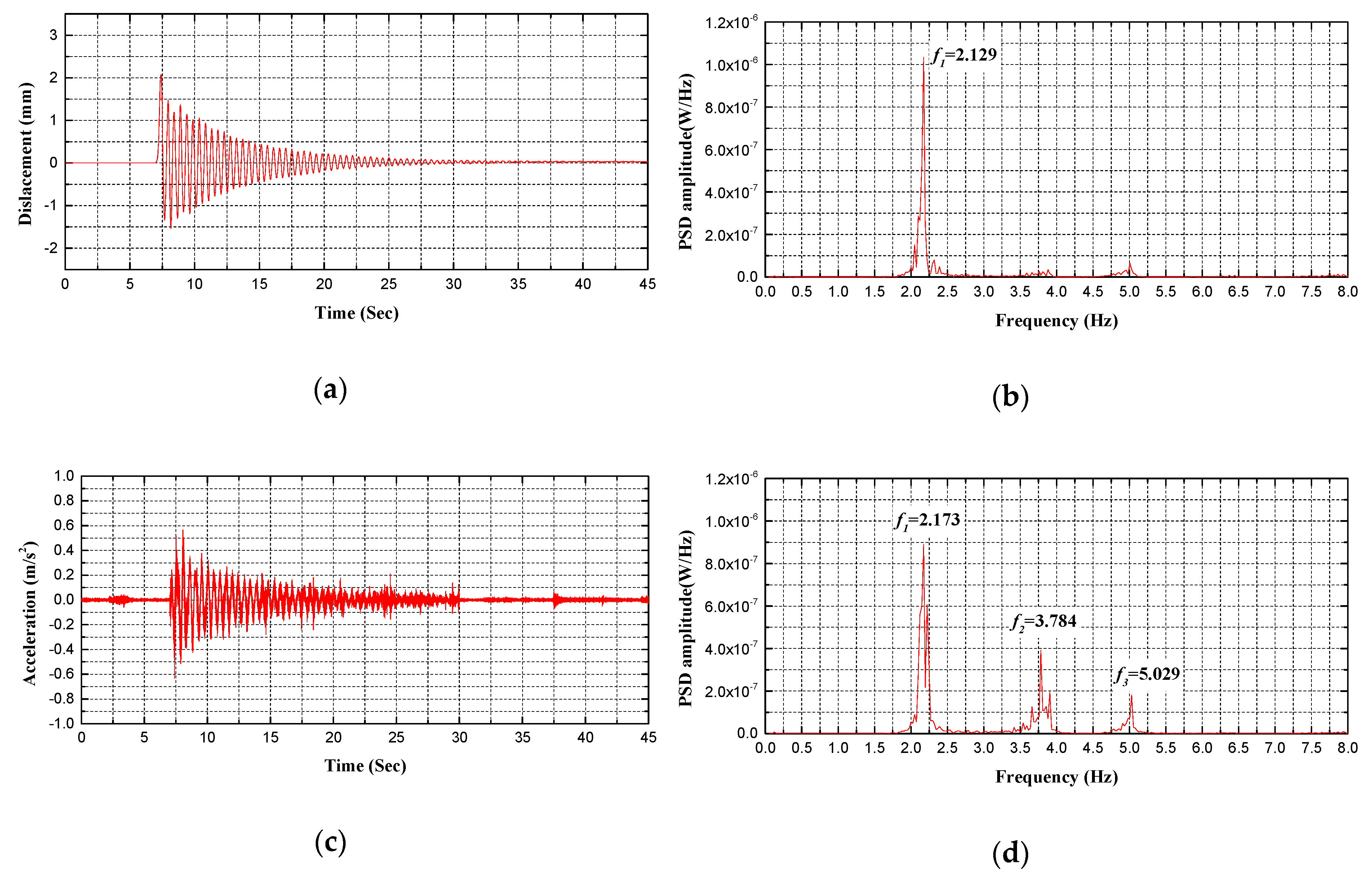
| B1 | Holographic Visual Sensor | 2.129 | - | - | - |
| Accelerometer | 2.173 | 3.784 | 5.029 | - | |
| B2 | Holographic Visual Sensor | 2.291 | - | - | - |
| Accelerometer | 2.329 | 3.442 | 5.029 | - | |
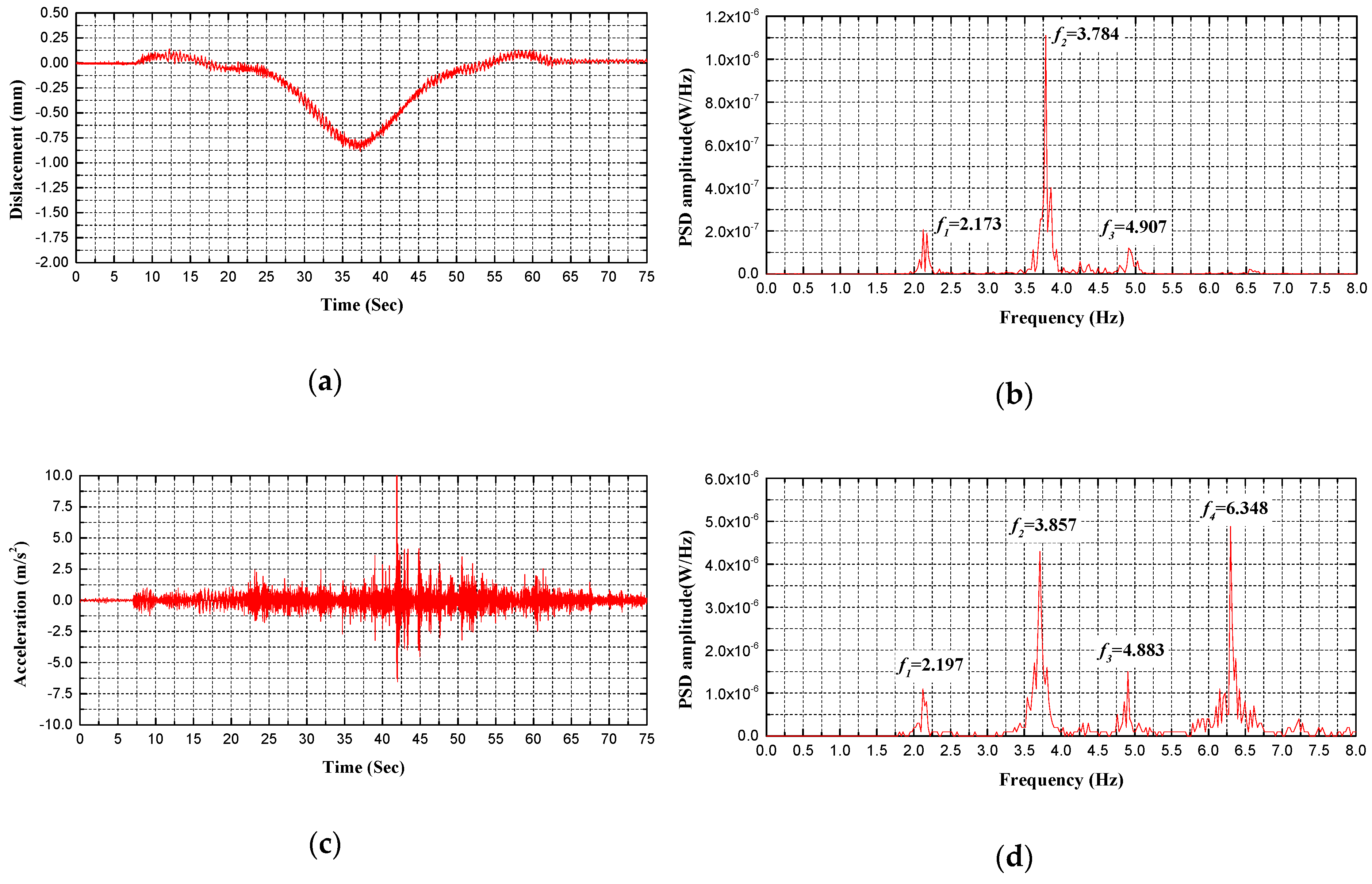
| C1 | Holographic Visual Sensor | 2.173 | 3.784 | 4.907 | |
| Accelerometer | 2.197 | 3.857 | 4.883 | 6.348 | |
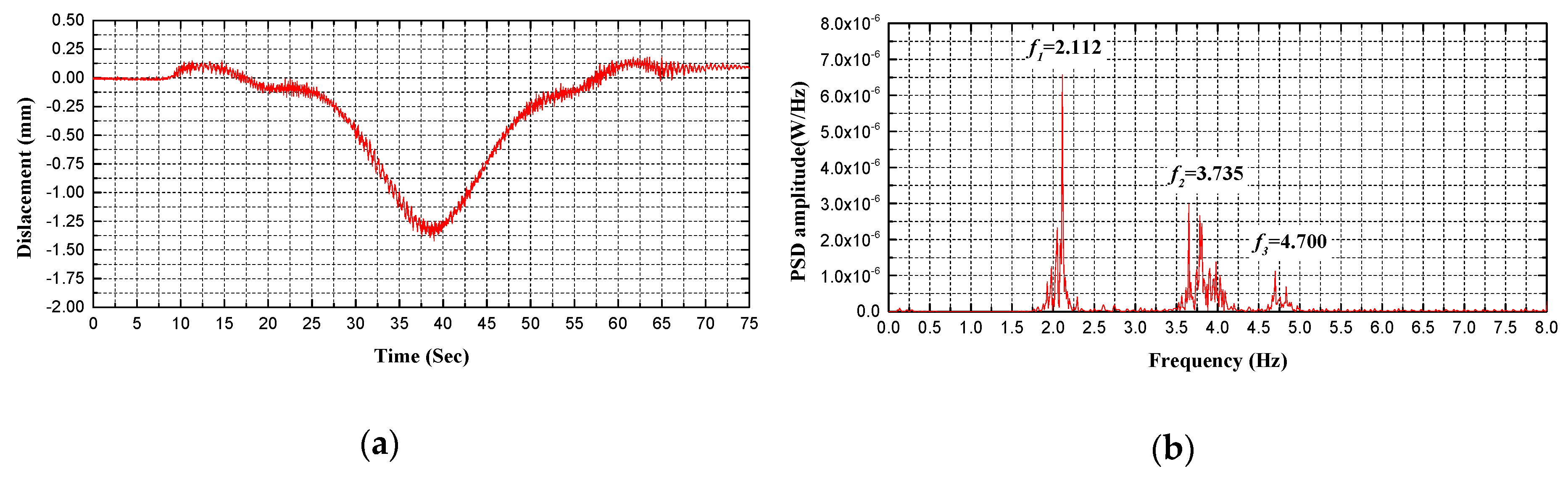
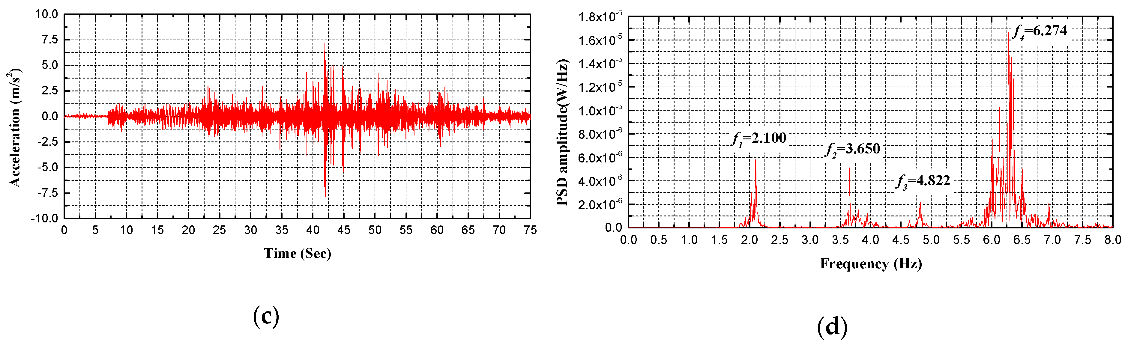
| C2 | Holographic Visual Sensor | 2.112 | 3.735 | 4.700 | - |
| Accelerometer | 2.100 | 3.650 | 4.822 | 6.274 | |
© 2020 by the authors. Licensee MDPI, Basel, Switzerland. This article is an open access article distributed under the terms and conditions of the Creative Commons Attribution (CC BY) license (http://creativecommons.org/licenses/by/4.0/).
Share and Cite
Shao, S.; Zhou, Z.; Deng, G.; Du, P.; Jian, C.; Yu, Z. Experiment of Structural Geometric Morphology Monitoring for Bridges Using Holographic Visual Sensor. Sensors 2020, 20, 1187. https://doi.org/10.3390/s20041187
Shao S, Zhou Z, Deng G, Du P, Jian C, Yu Z. Experiment of Structural Geometric Morphology Monitoring for Bridges Using Holographic Visual Sensor. Sensors. 2020; 20(4):1187. https://doi.org/10.3390/s20041187
Chicago/Turabian StyleShao, Shuai, Zhixiang Zhou, Guojun Deng, Peng Du, Chuanyi Jian, and Zhongru Yu. 2020. "Experiment of Structural Geometric Morphology Monitoring for Bridges Using Holographic Visual Sensor" Sensors 20, no. 4: 1187. https://doi.org/10.3390/s20041187