2.1. Methodology
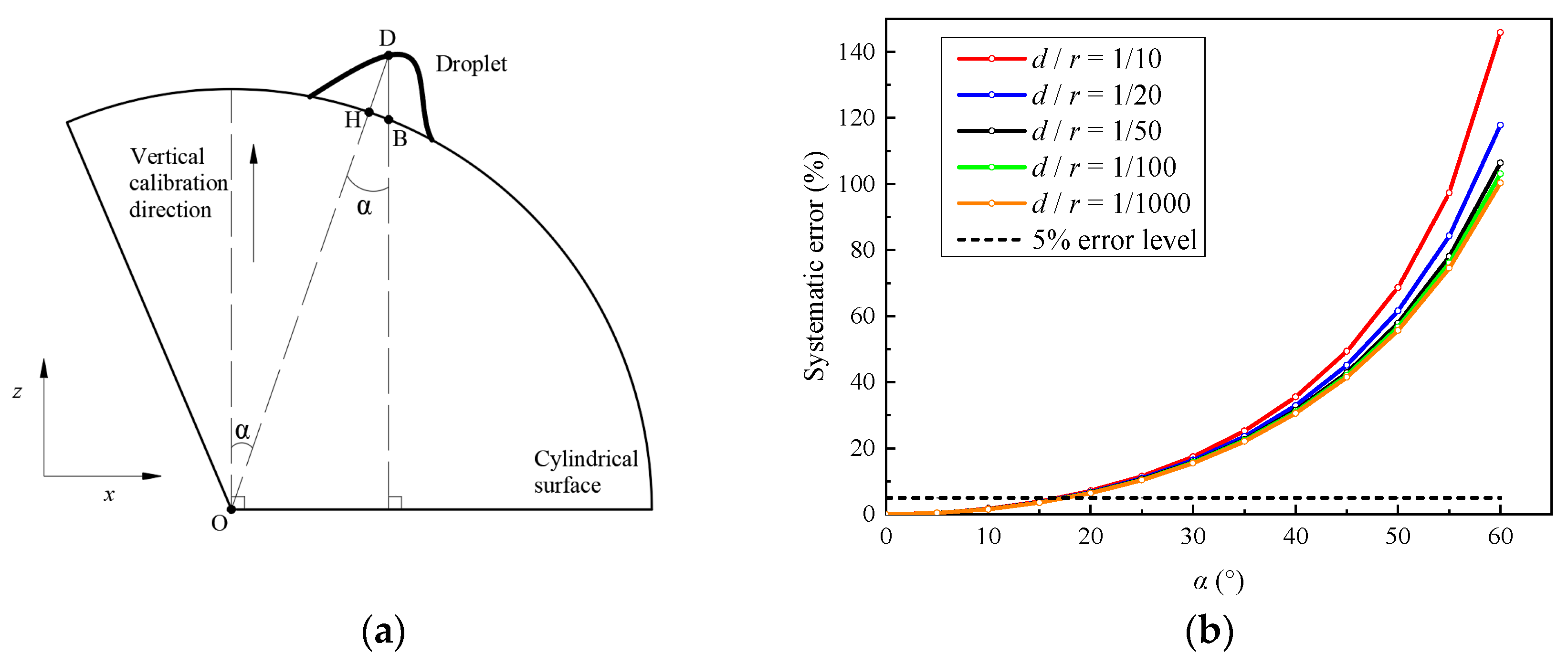
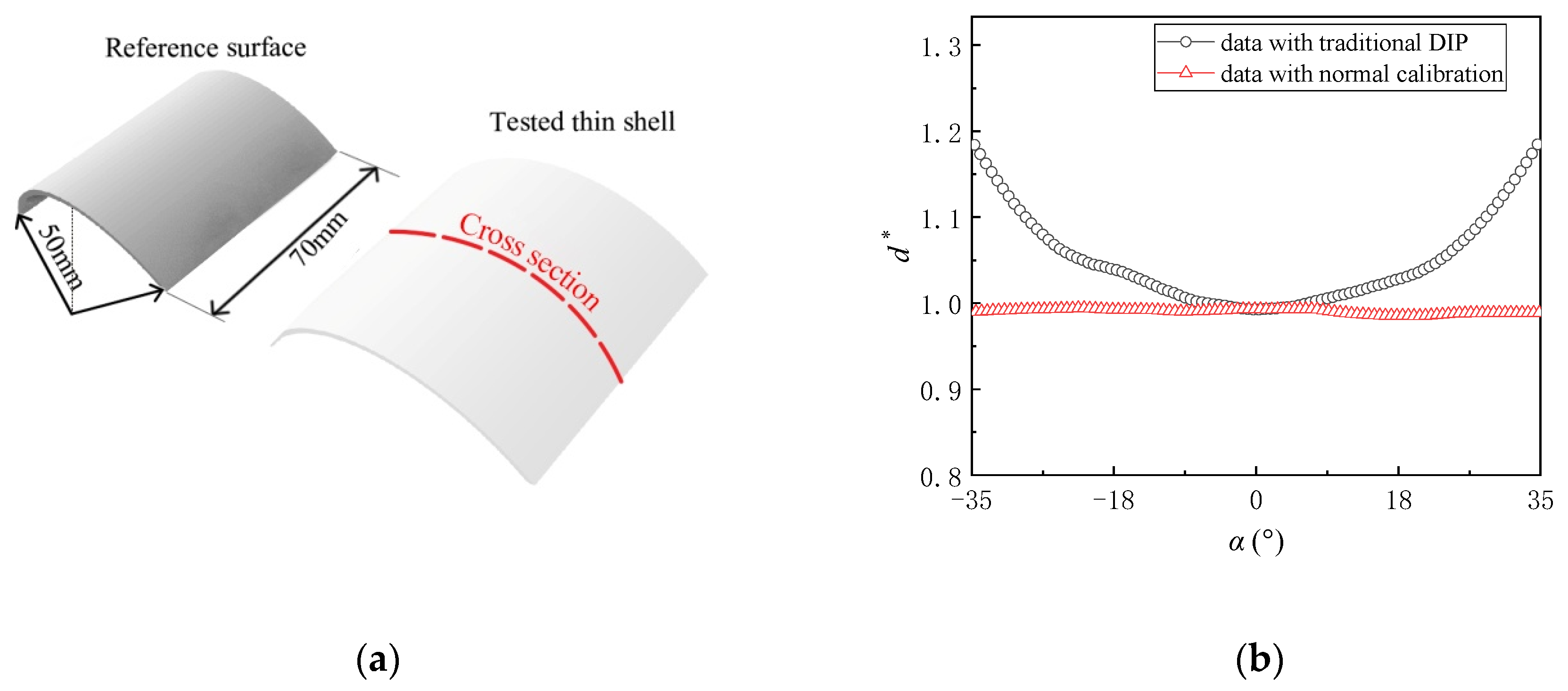
For the measurement on a curved surface (as shown in
Figure 2a), if the preceding vertical calibration is still adopted, the measured thickness
will be in the vertical direction. However, the real thickness of the droplet is
, which is normal to the surface. Obviously, as illustrated in
Figure 2b, the systematic bias between
and
depends on the included angle α between them. With the increase of
α, the systematic bias raises quickly. Moreover, the ratio of the real thickness
d (
) and the local radius of the curved surface
r also contributes to the systematic bias. This effect will be magnified when
α becomes larger. That is, the traditional DIP overestimates the thickness of droplets on a curved surface. If the accepted error level is 5%, the traditional DIP technique must be improved to eliminate this systematic error when
α is larger than 17°, even when
d/
r approaches zero.
Consequently, a correction coefficient
(=
) is necessary to eliminate the above-mentioned bias for applying the DIP technique on a curved surface.
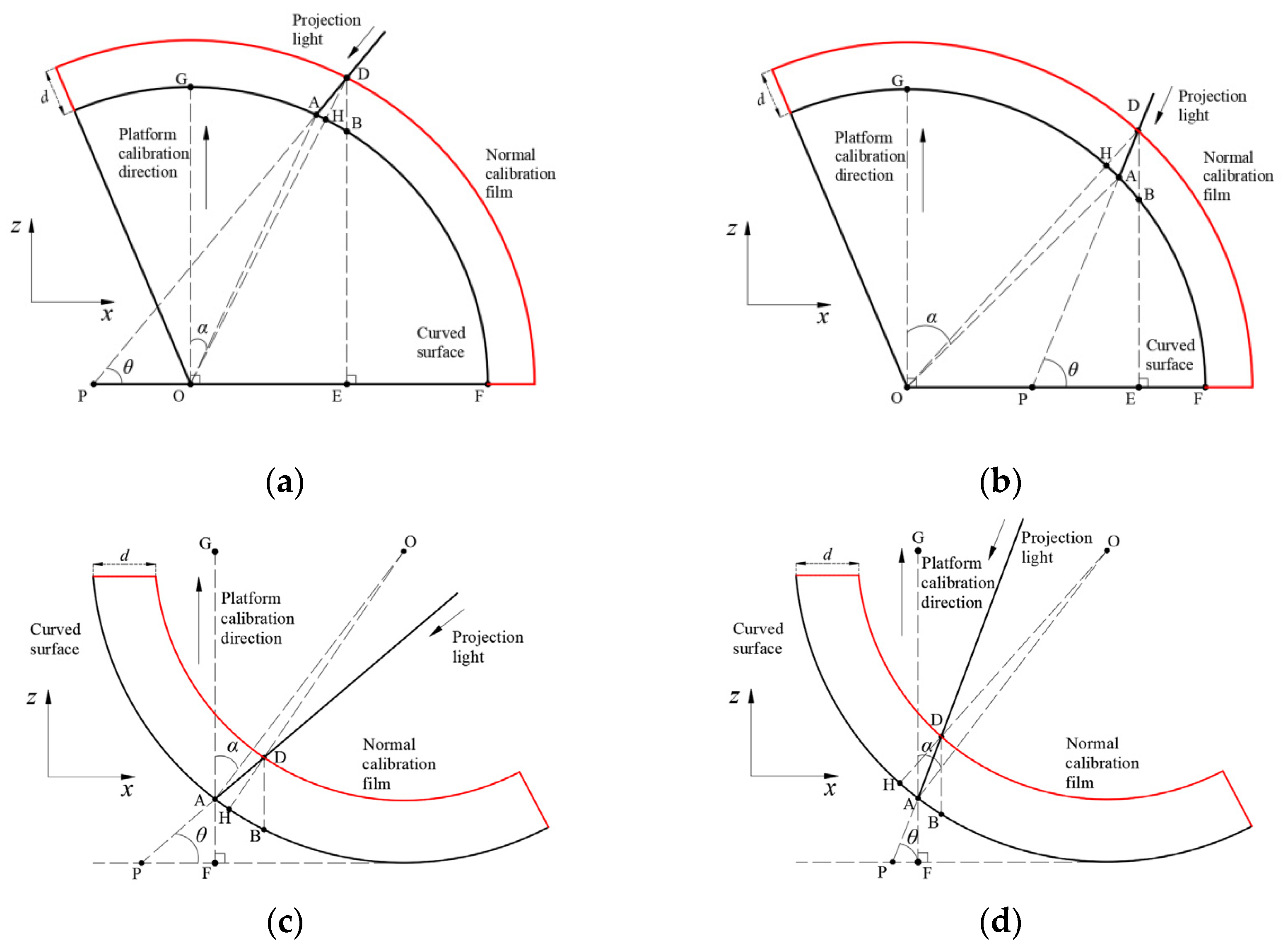
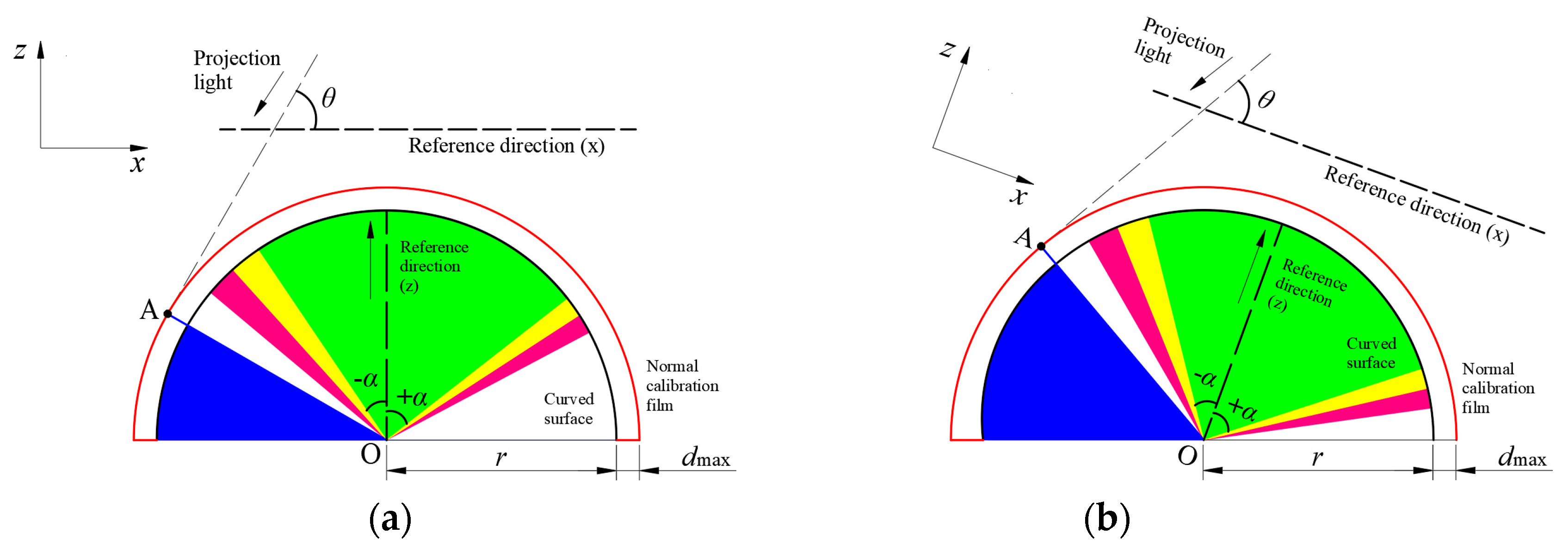
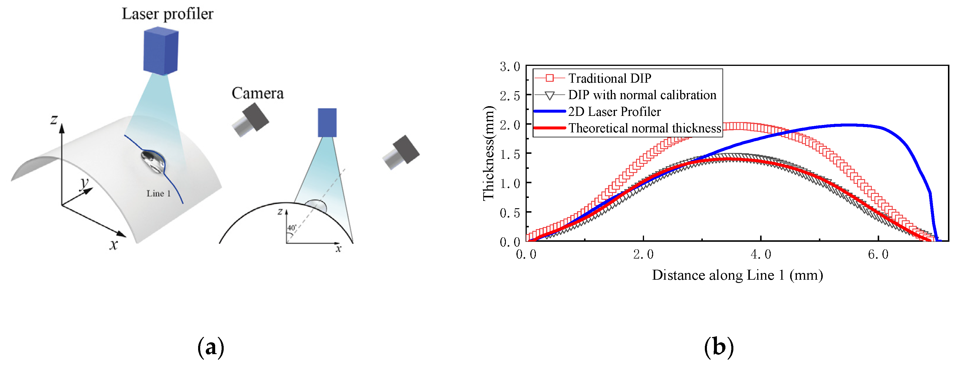
Figure 3a shows a typical geometric configuration of the DIP measurement on a curved surface. The projected light falls on an arbitrary curved surface at point A with an angle
θ. The angle between radius
and the vertical direction,
, is
α. It should be mentioned that
α can be negative when the projected light falls on the left side of
.
If the original curved surface expands to its new position with a normal displacement of
d (
, as shown in
Figure 3a. Assume that the radius of the curved surface
r is much larger than
d. Under the condition of 90°−
α ≥
θ, the thickness
, acquired by the previous vertical calibration procedure, can be calculated by Equations (3)–(5):
According to the law of sines:
Because
and
, thus:
Hence, Equation (6) can be simplified according to Equation (7) as follows:
Based on the discussion above, in a certain interrogation window on the surface (i.e., r, α and θ are constant), the thickness, , is only determined by the normal displacement, d. Meanwhile, the correction coefficient (=) can be also determined.
Figure 3b–d present the other three possible configurations for the application of the DIP measurement on a curved surface. Based on similar analysis procedure,
k2 for these configurations can all be determined.
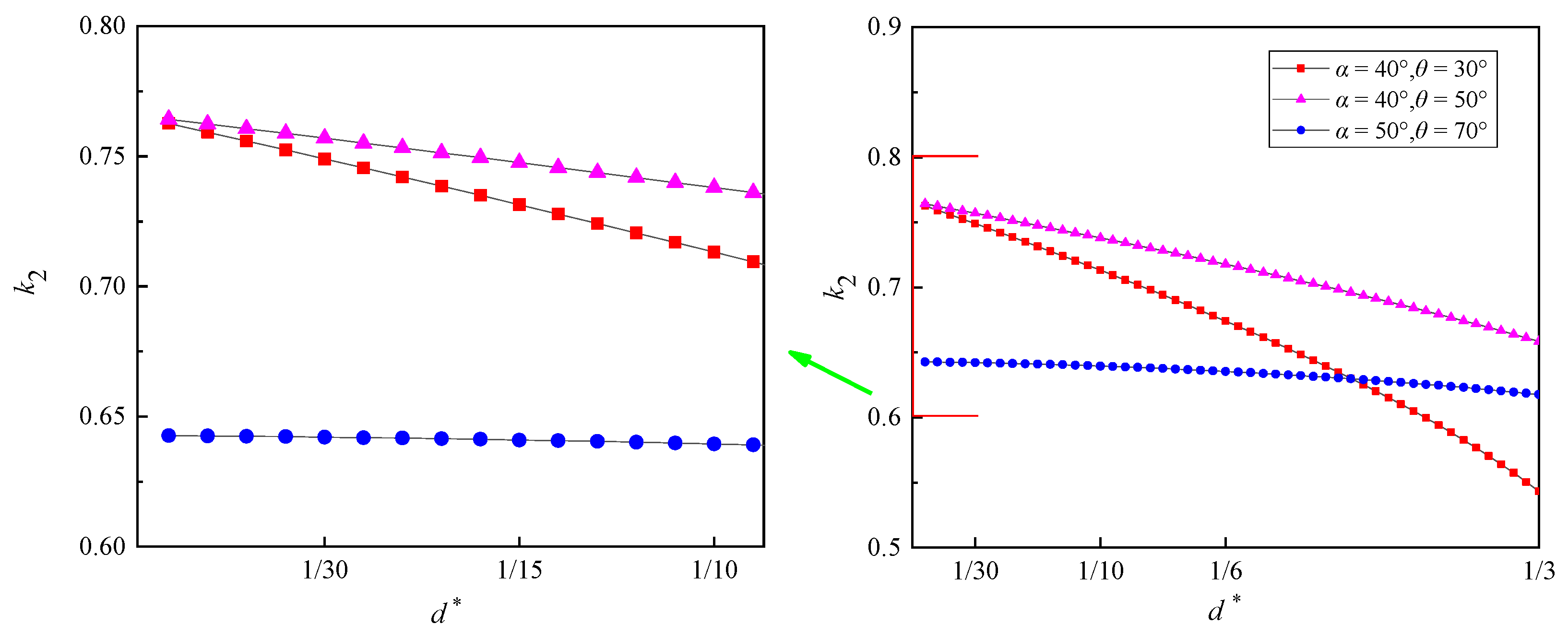
Figure 4 illustrates the relationship between
d* (normalized with the local radius of the curved surface
r) and
k2, calculated from Equations (3)–(8).
k2 decreases gradually with the increasing
d*. Obviously,
and
d* show good linear relationship when
d* ranging from 0 to 0.1.
Assume that the linear relation between
d* and
k2 is:
where
is normalized with the local radius of the curved surface
r.
According to Equation (2), Equation (9) can be expressed as:
In a certain interrogation window on the surface,
k1 is a constant (Zhang et al. [
12]). Hence, Equation (10) indicates that
and
d are also quasi-linearly correlated. Thus, it is acceptable to get the
relation by measuring
at only two specific
d.
If we can attach two shells with given thickness to the curved surface, respectively, then the linear relation between
and
d can be acquired. This calibration is named for “normal calibration” hereafter in the present paper. It can be obtained:
In Equation (11), the distance between the two images can be determined based on cross-correlation between the tested images and reference image. The constant coefficients k1C3 and k1C4 can be calculated by normal calibration procedure. Hence, the normal displacement, d, can be also computed by Equation (11).
2.2. Error Analysis
The
in normal calibration is assumed to be perfectly linear. The systematic error caused by this assumption is related to
α,
θ and the ratio of
dmax (the maximum normal displacement) and
r. By optimizing the setup arrangement, e.g.,
α and
θ, this systematic error can be controlled within an acceptable level.
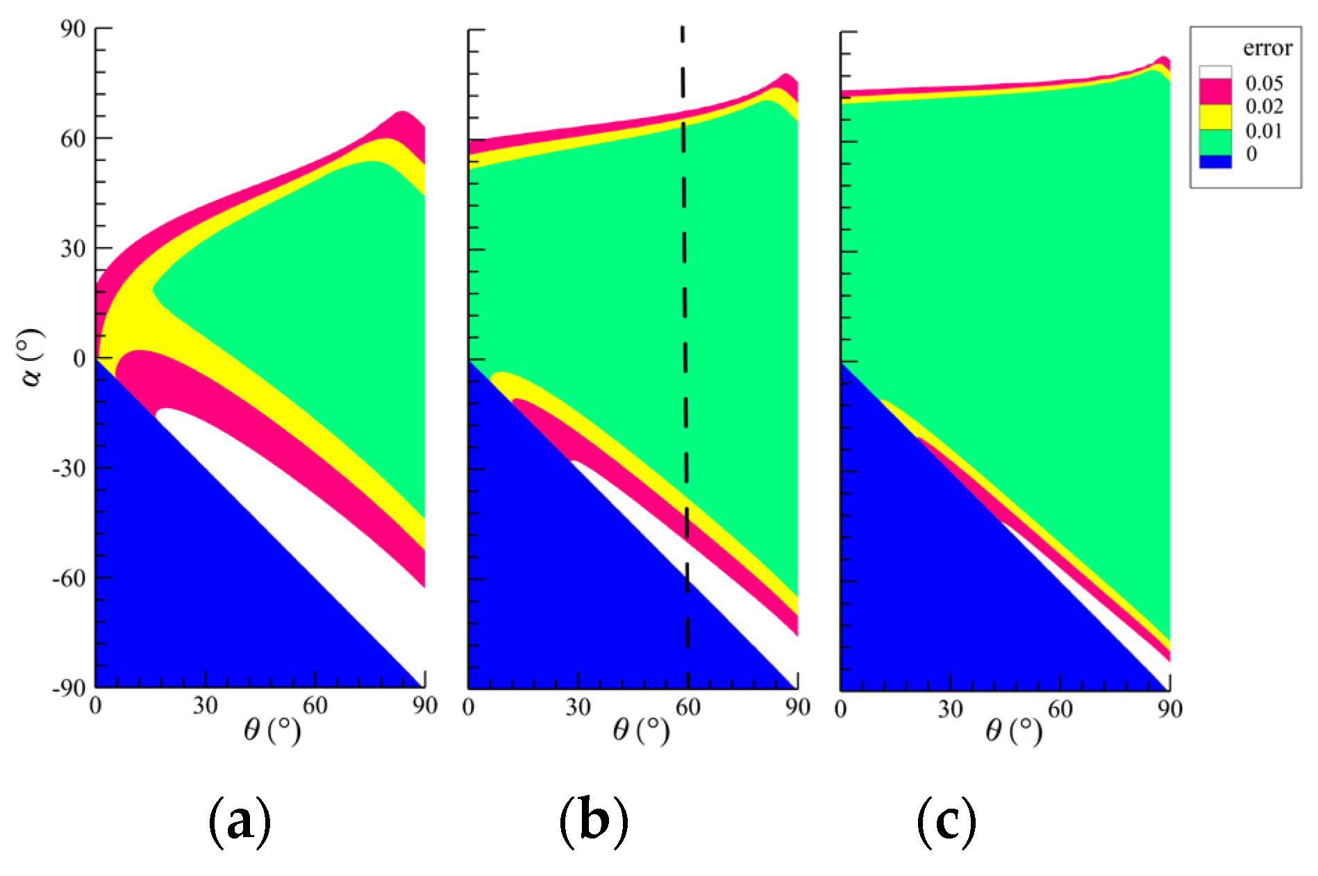
Figure 5 shows the dependence of this systematic error on the two main influencing factors
α and
θ for different
r and
dmax. The thickness of two hypothetical shells for normal calibration is set as
and
.
For better illustration,
Figure 6 displays the systematic error under the condition of
dmax/
r =
,
= 60°, marked with the black dashed line in
Figure 5b. Note that, as shown in
Figure 3,
θ is determined by the position and the incidence angle of the projector and
α represents the location of the interrogation window to be tested. As expected, both
α and
θ have obvious effects on the systematic error. In
Figure 6, the blue region on the left side of OA is out of the field illuminated by the projected light. Based on the information provided by
Figure 5 and
Figure 6 and Equation (1), the projector should be mounted far away from the reference surface. Meanwhile, in order to obtain a larger green area, the recommended angle
is about 80°. Moreover, rather than the standard reference axis (vertical direction and horizontal direction) reported by Zhang et al. [
12], as shown in
Figure 6a, the reference axis can be adjusted arbitrarily, making the tested region within the green area in order to obtain precise results.
Likewise, the ratio of
dmax and
r also has remarkable influences on the systematic error. According to
Figure 5, the systematic error reduces with the decrease of the ratio of
dmax and
r and vice versa.
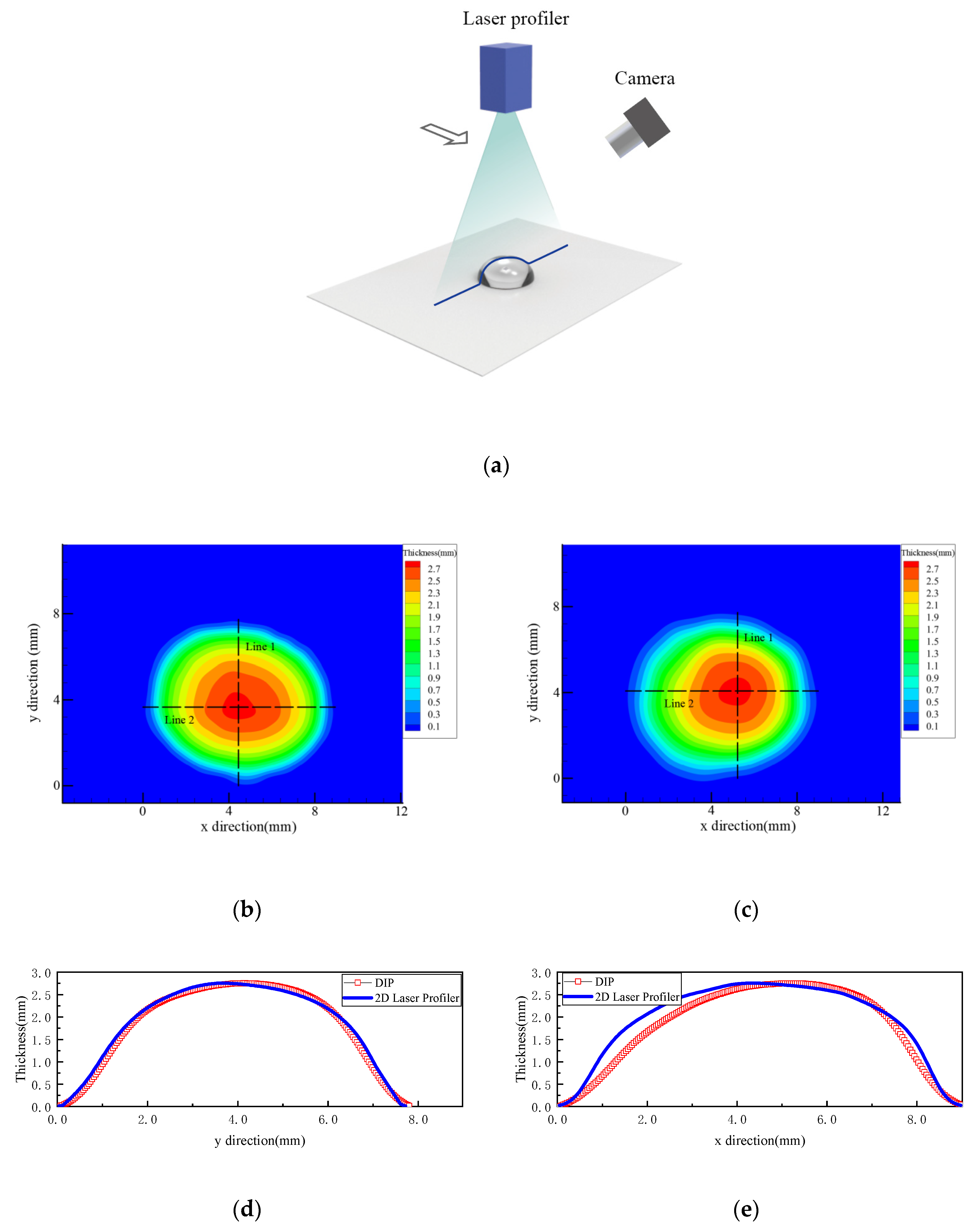
2.3. Experimental Setup
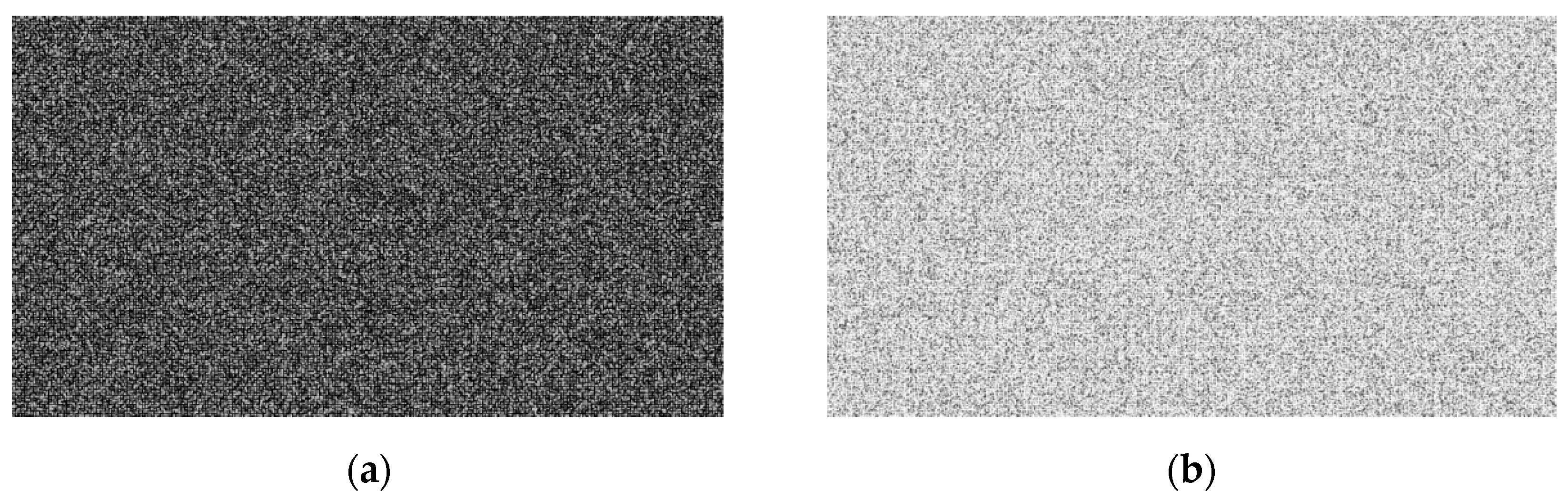
A grayscale image consists of particles with random gray values generated by Matlab was used as the projected image, as shown in
Figure 7. The gray level of this projected image should be adjusted according to the ambient lighting condition. Because the combined effects of intense ambient lighting condition and high gray level may lead to the improper focusing of the camera. Thus, it is recommended that the experiments are conducted in a dark environment. Meanwhile, the gray level of the projected image should not be too high.
In the present experiment, a digital projector (Robot go 3D, produced by Aiteqi Technology Company Limited, Shenzhen, China; the resolution was 1280 × 800 pixel2) was used to cast the random scatter particle image onto a reference surface for the DIP measurement. And a digital single-lens reflex (DSLR) camera (Canon EOS 6D, produced by Canon Company Limited, Tokyo, Japan; the highest resolution was 5472 × 3648 pixel2, the valid pixel was 20 million) was applied for capturing images. The measured surface was one-third of a cylindrical surface with the length of 70 mm and radius of 50 mm. It was produced by a rapid 3D prototyping machine using white resin material and carefully polished. Two normal calibration shells, with the thickness of 1 mm and 2 mm, respectively, were prepared.
A high-resolution 2D Laser Profiler (Keyence LJ-G200, produced by Keyence Corporation, Itasca, IL, USA; the length of the linear laser was 62 mm, the accuracy was up to 2 μm) was also used to measure the thickness of the droplet, which provided the validation for the present DIP technique.
The normal calibration procedure can be divided into the following steps:
Based on the measurement region, fix the projector and camera according to the result shown in
Figure 5 and
Figure 6.
Project the image onto the tested curved surface. Take a picture of the projected image without water droplet or rivulet, which will be used as “original image”.
Attach the two thin shells with given thicknesses to the measured surface, respectively. Take pictures of the projected image on each of the two shells. These two pictures will be used as “normal calibration images”.
Remove the thin shells. Make droplets or rivulets attached on the surface. Then, the projected image will be distorted with the appearance of these water droplets or rivulets. Capture the distorted images, which contain the geometric information of the water droplets or rivulets.
Calculate the constant coefficients k1C3 and k1C4 with cross-correlation between the “normal calibration images” and “original image”.
Calculate the thickness of water droplets or rivulets with cross-correlation between the distorted images and “original image”
Noted that, in order to enhance the contrast of the projected image on the free surface of the water droplet, a very small amount of titanium pigment should be added into the water.
2.4. Interrogation Window Size
The interrogation window (IW) size does influence the measurement results. For the present experiment, the resolution of the camera was 5472 × 3648 pixel2 (which was not completely used for cross-correlation, only the part containing the droplet was adopted for the measurement), each pixel indicates 0.05 mm. The cross-correlation algorithm provides one result for each IW according to the image displacement within it. It was similar to a spatial filtering or average for each IW. Thus, a larger IW reduces the spatial resolution of the measurement. However, if the IW is set to small, the cross-correlation algorithm may not provide a reliable result, because the image within each IW is too small to provide enough information for cross-correlation. The smallest applicable IW largely depends on the quality of the image captured.
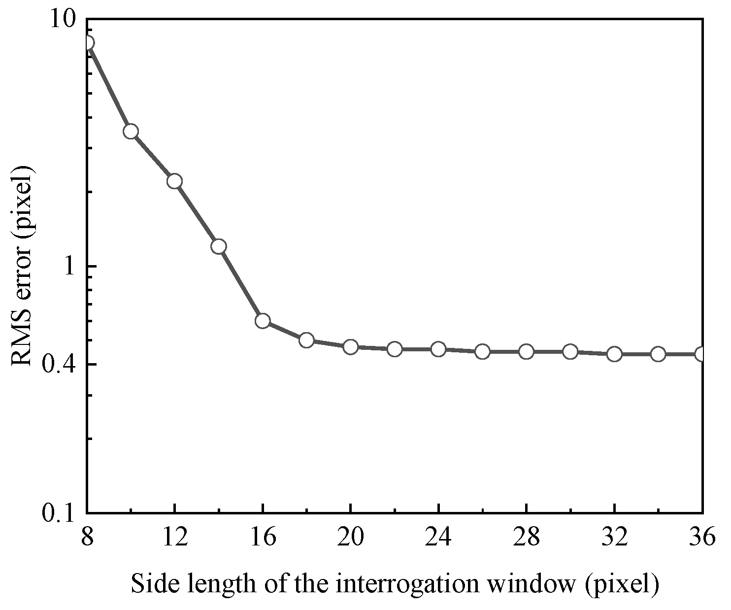
For the present experiment, the effects of IW on the results were tested during calibration process. Since the thickness of the calibration shell was given and uniform, the cross-correlation was conducted for different IWs and their corresponding RMS values were calculated, as shown in
Figure 8. As expected, the Root Mean Square (RMS) value reduces quickly with increasing the size of IW and becomes stable for the IW larger than 18 × 18 pixel
2 (0.9 × 0.9 mm
2). Consequently, the IW of 18 × 18 pixel
2 was utilized in the experiment.


