3.1. Optical Losses from Tapers and Beam Profiles
Several heating and elongation tests were carried out with pulling rate varying from 0.5 to 13 mm/min, while keeping the oven either stationary or moving at a rate of 5 to 15 mm/min over a distance of 20 mm. The pulling rates were determined by two parameters: (i) the initial tendency of the fiber to contract, due to memory processes in the PMMA which set the lower pulling limit and (ii) braking of the fiber when the pull rate exceeded the rate at which the fiber-core dropped below T
g. The taper lengths ranged from 6 mm to 17 mm and formation of asymmetrical conical sections were observed when only one stage was allowed to move. As mentioned above, tapers drawn near T
g and at about 350 to 400 μm/min at temperatures of 125 to 135 °C, became lossy, radiating from the conical section (
Figure 4a). The intensity variations along the taper length are depicted in
Figure 4b, with most of the light exiting midway of the conical section indicating that the modes were no longer guided in the taper but radiated in nearly 2π steradians.
The physical dimensions of the tapers were measured from the shadowgraphs using Image-J. The length of the conical sections was defined as the points were the diameters at the thin and thick sections were respectively, 10% and 90% of the final values, and ranged from 6 to 17 mm. The corresponding conical angles were from 1.0 ° to 2.5° and waists diameters from 30 to 90 μm with a typical profile shown in
Figure 5.
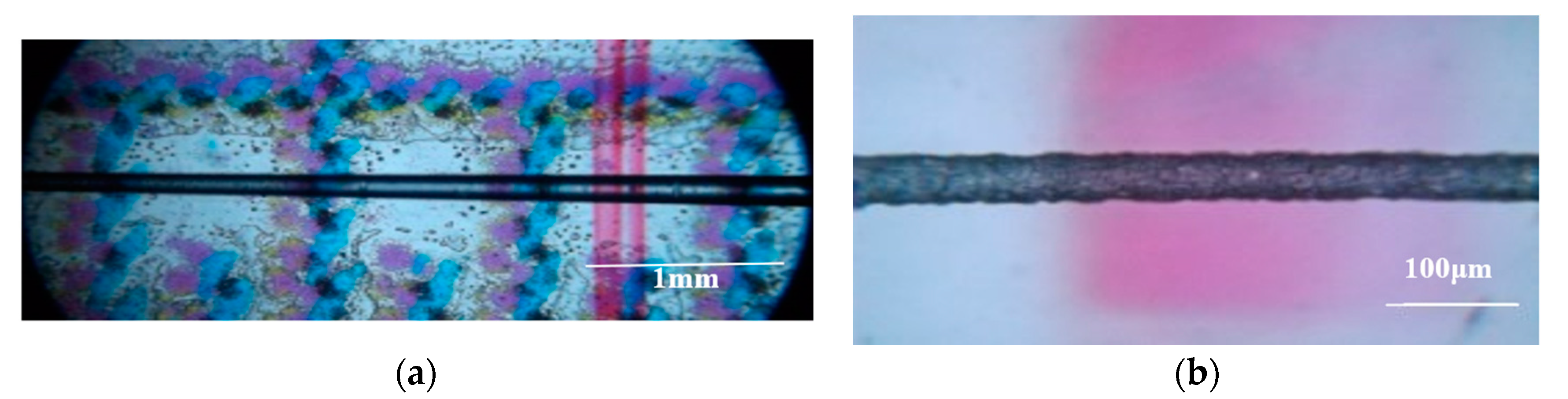
Under an optical microscope, the bi-conical fiber tapers exposed surface imperfections (i.e., anomalous surface, AS). In
Figure 6a,b, a 3 mm conical section and a section near the tip of the taper with diameter of about 35 μm, are shown respectively. The length of AS did not cover the entire taper (
Figure 6a) but progresses in the thinner sections covering a few mm in the down-taper, extending into the taper waist, covering 40% to 50% of the taper length. By correlating the lengths of AS on the conical surfaces of the tapers with the intensity profile measured with Image-J (
Figure 6b), it was apparent that optical loss coincided with the AS region. This finding verified that the output modes were no longer guided by Total Internal Reflection (TIR) but undergone diffuse scattering by AS. Furthermore, light was diffused out of the taper well before the end the AS region.
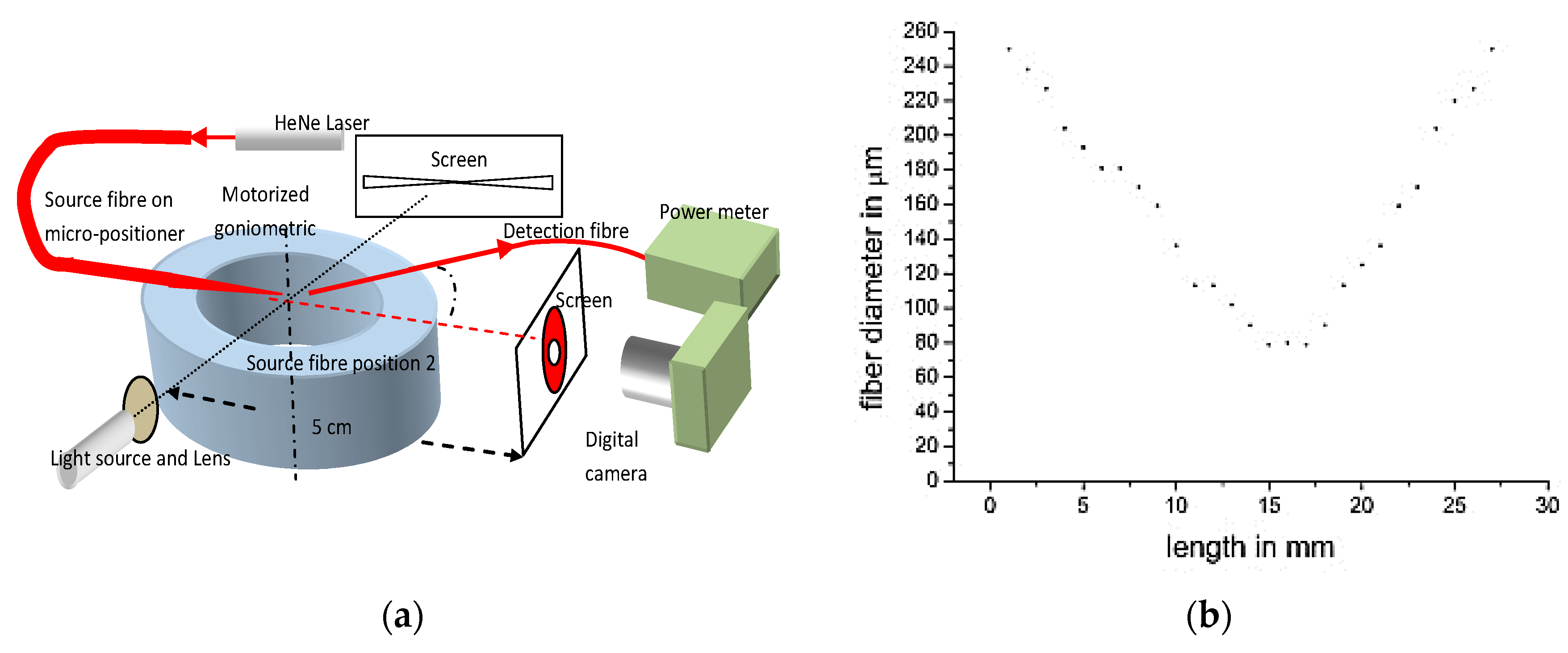
The output modal intensity profile from the tapers were measured using the goniometric set up, as described earlier in
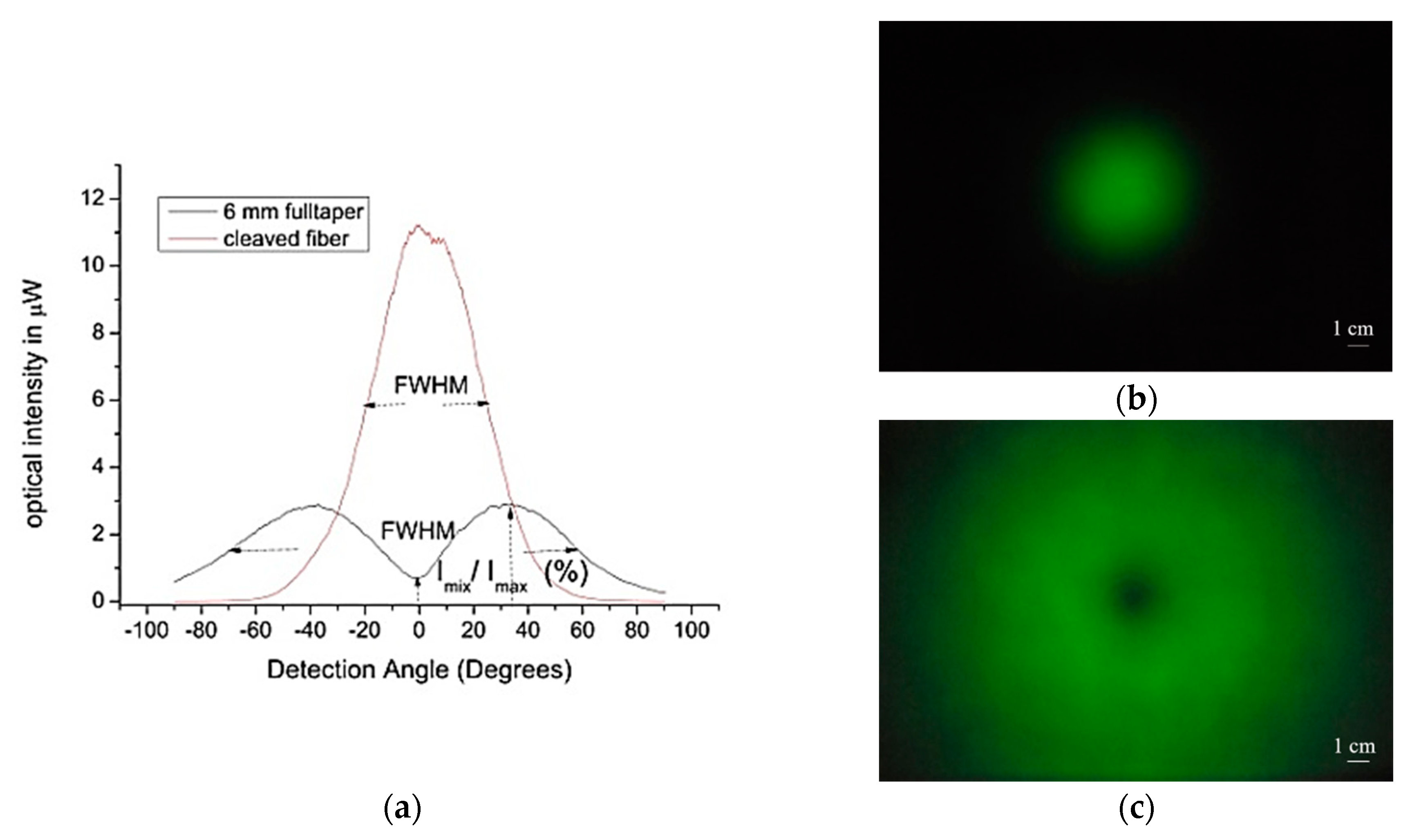
Figure 2, together with the beam profile from a flat polished fiber, used for comparison. Typical goniometric beam profiles for a polished fiber and a taper are shown in
Figure 7a. The modal intensity profile from a polished fiber and a typical 15 mm long taper were projected on a 25 cm by 17 cm semi-transparent screen and photographed with a digital camera (
Figure 7b,c).
The “effective” diameter of hollow beams was measured at the full width half maximum (FWHM), with the maximum being defined relative to the average intensities of the twin peaks, as indicated in
Figure 7a. The goniometric measurements for normal 250 μm diameter polished fibers with NA of 0.38 were compared with measurements of a typical 6 mm long fiber taper with cone angle of about 1.2°, yielded a FWHM values of 45° and 130°, respectively. Similarly, the central intensity-depression (ID), or dark spot, was measured as the percentage ratio of the intensity at the center, relative to the average intensities of the twin peaks (
Figure 7a).
3.2. Background on Beam Profiles from MMF Tapers
To better understand the origin of the side losses it is necessary to model the expected exit angles from a long smooth MMF taper using the meridian ray optics model. In this first approximation model, the paraxial modes are not included (a) due to the large diameter of the fibers and (b) because the Gaussian modal intensity profile implies the light energy is concentrated in the center of the beam (
Figure 7b). Therefore, ray-optics theory applied on meridian rays can adequately describe the light propagating in the large core fiber tapers and predict the formation of hollow beams with low exit angles in the conical section of the taper [
16]. When calculating ray optic paths in the fiber, cladding modes can be neglected due to very thin cladding in the conical section of the taper. In
Figure 8, meridian rays enter a taper with cone angle
α, undergoing successive total internal reflections (TIR), which gradually reduce the reflected angle at the interface. Eventually the rays will exceed the critical angle and will be converted to cladding modes refracting out of the fiber taper as radiation modes [
16,
17,
18]. If we consider a meridian ray guided in the conical section, the reflected angles at the interfaces, R
1, R
2, ..., R
m, change as shown schematically in
Figure 8. At the interface, the rays’ angle can be calculated for an initial angle θ
1 as:
where m = 1, 2, 3 …, are the number of successive reflections at the taper boundaries.
Consequently, the optical transmission intensity can be modeled for a long taper. Typical results in polar coordinates are shown in
Figure 9 with cone angle
α ranging from 1° to 3°. This theoretical model ignores the thin cladding which eventually becomes even thinner by the drawing process shortening the optical paths. Therefore, the model predicts that when shaping a hollow beam, most of the light escapes from the sides of the smooth taper in angles 5° to 17° to the fiber axis while no light exits from the tip of the fiber (
Figure 9).
However, the calculated profile of beam is much narrower than the experimental, as depicted in
Figure 7, with exit angles of the two peaks at about ±45° to ±50°, corresponding to a much wider hollow beam profile. This discrepancy is attributed to the AS, which changes the beam profile due to diffuse scattering at the surface of the taper and cannot be included in the theoretical model. Although it is beyond the scope of this work, the formation of the AS can be attributed to the differences in dopants levels required for the refractive indices of the core and cladding, that result in varied T
g [
18]. An alternative explanation could be deferential heating due the heater geometry and the size of the slot. During drawing at T
g = 130 °C, the two layers undergo different relative motion leading to the AS which increased optical losses from this region of the taper.
Experimentally, two parameters are used to characterize the hollow beam profile, namely the FWHM of the tween peaks and the ID of the beam. A positive correlation of the A.S length with the beam profile is shown in
Figure 10a. Furthermore, the depth of ID was negatively correlated to AS length as shown in
Figure 10b. Based on these results the ID % values of the hollow beam, decrease with the length of the AS. For example, 3 mm length of AS corresponds to ID of 28% of average peaks values while reducing to about 16% when the AS length increases to 4.5 mm. Therefore, as the length of the AS increases up to 4.5 mm, more light exits from the side of the taper generating of a hollow beam with ID as low as 3%. This was also verified by the low throughput transmission (less than 1%), measured before cutting the biconical tapers into two single tapers.
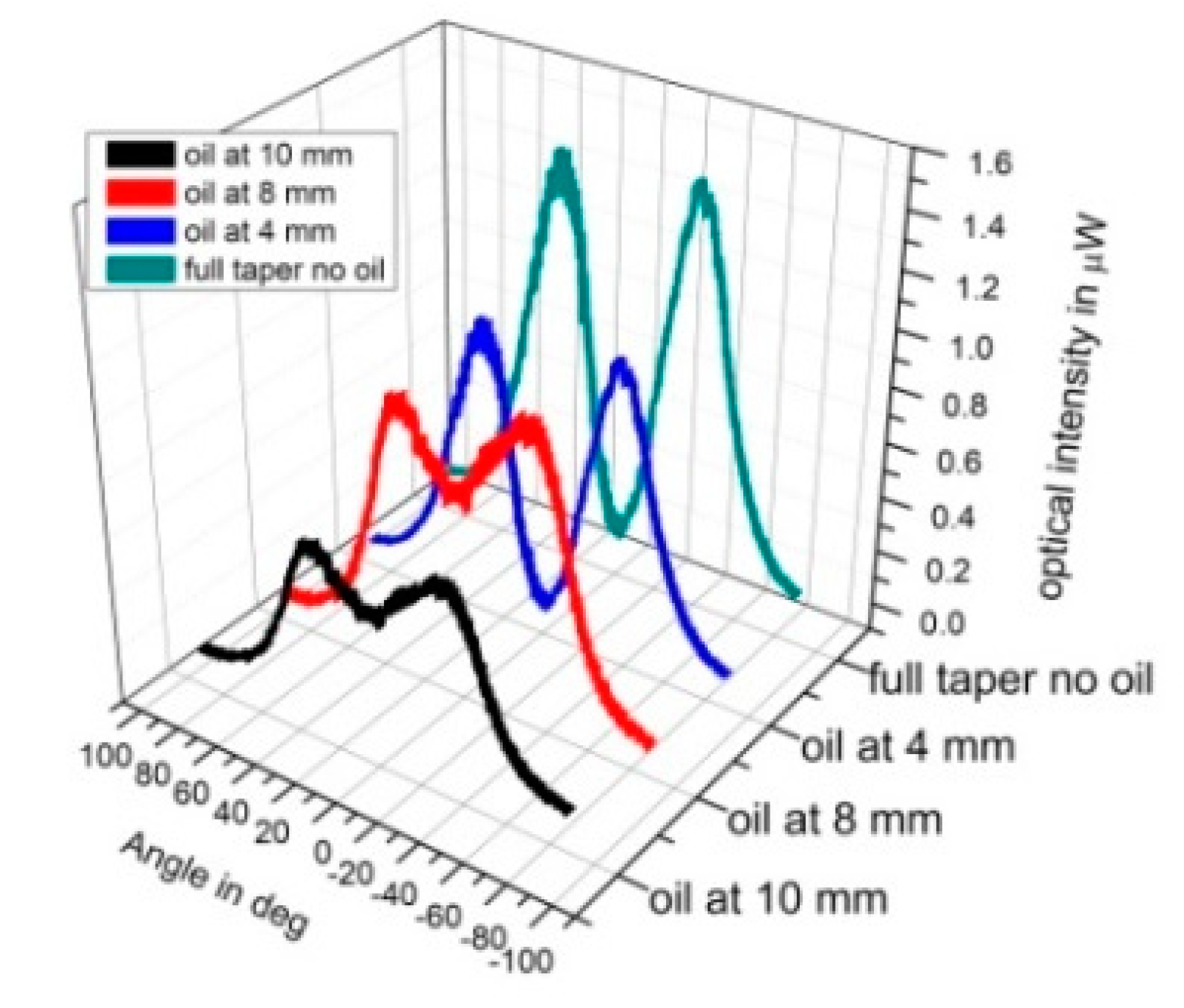
To further investigate the loss mechanism in tapers, the AS region was effectively “smoothed” by covering it with index matching oil with refractive index
n = 1.51. Using a small hyperemic needle, an oil droplet was progressively dragged along the surface of the conical section starting from the tip until all the AS was covered.
Figure 11 shows the change to the hollow beam profile, for a 13 mm long taper with about 10 mm of AS, which is progressively covered with oil. As expected, when oil was applied upon AS, scattering is gradually reduced and more light reaches the end of the taper, shaping a beam profile with reduced ID of the central dark spot.
Specifically, for the full taper the ID is about 3% of the average twin-peak values, gradually increasing to about 75 % when the oil covers the entire AS region. Similarly, the FWHM of the beam is also gradually reduced, due to less scattering from the conical section, reaching lower exit angles of 10° to 17°, when the AS is completely covered, which are close to the predicted values of a smooth taper as predicted by the theoretical model (
Figure 9).
3.3. Beam Expansion with Cutback
Based on the above results it is evident that the AS on the surface of the taper, causes diffuse optical transmission of the guided modes to exit the taper, changing the optical profile of the beam. In order to quantify this effect further and to investigate the ability to alter the hollow beam profile, the length of the AS region of the taper was gradually shortened. This involved cutting progressively small sections of the taper (cutback), thus altering the ratio of light exiting the side and the cleaved end-facet of the taper, as shown in
Figure 12 where the AS length was reduced, allowing the more central guided modes to exit the fiber cleaved-end rather than the side of the taper.
Using the experimental setup outlined in
Figure 2a, the taper was placed in the center of the goniometer while the rotating arm was scanning from ±90°. Once the angular scan was completed, a small section of 0.5 mm long was cleaved, and the fiber tip repositioned in the center of rotating setup. The angular measurements repeated until the conical section was completely removed. In
Figure 13a, a 3D graph of the angular intensity variations is shown for progressive cutbacks of the taper. For a 6.4 mm long taper, the initial hollow beam profile changed to an expanded Gaussian, and near top-hat when the taper length was reduced to about 3.9 and 2.8 mm, respectively, reverting gradually to Gaussian when all the taped sections together with the AS were removed.
The normalized intensity variations as a function of angle for three distinct cutback lengths are depicted in
Figure 13b. The black line is for the full taper of 6.4 mm, with the ID having its lowest value of about 17% and effective FWHM of the hollow beam is widest at about 128°. The red line is for the taper shortened to 3.9 mm; the beam is no longer hollow exhibiting a wide profile with FWHM, extending to nearly 100°. The blue trace is the beam profile when the entire taper was cut off with a FWHM of about 45°, corresponding to a fiber with NA of 0.38. The modeled angular distribution for a smooth taper is shown in the doted magenta trace and is similar to that in
Figure 9 expressed in linear rather than polar coordinates. The expected exit angle for this taper has FWHM of 32°. Finally, the variation in the FWHM with taper length during cut back, is shown in
Figure 14. As a result, with tapers in POF fibers, the beam profile can be tailored as necessary, expanding the normal FWHM of 45° to above 120°.
3.4. Ice Detection with High-NA POF Fiber Tapers
One important application of the discussed beam expansion technique is in the development of a fiber optics ice detector. Ice accumulates on the leading edge of aerodynamic surfaces disrupting the normal airflow and occurs when aircrafts fly through cold moist air. These conditions are particularly dangerous when an aircraft flies at low altitudes near congested airports because lift decreases and drag increases [
19,
20]. The current technology for ice detection relies on atmospheric conditions measurements like temperature, humidity, and liquid water content (LWC) in order to calculate icing conditions based on algorithms, and alert the aircraft of the ice conditions without directly detecting ice on the wings. Similarly, present icing sensors which are located on the nose of the aircraft, and are based on a vibrating wire which measures the ice mass accreting on the wire, through changes in its resonant frequency, also don’t detect ice directly on the wings [
21].
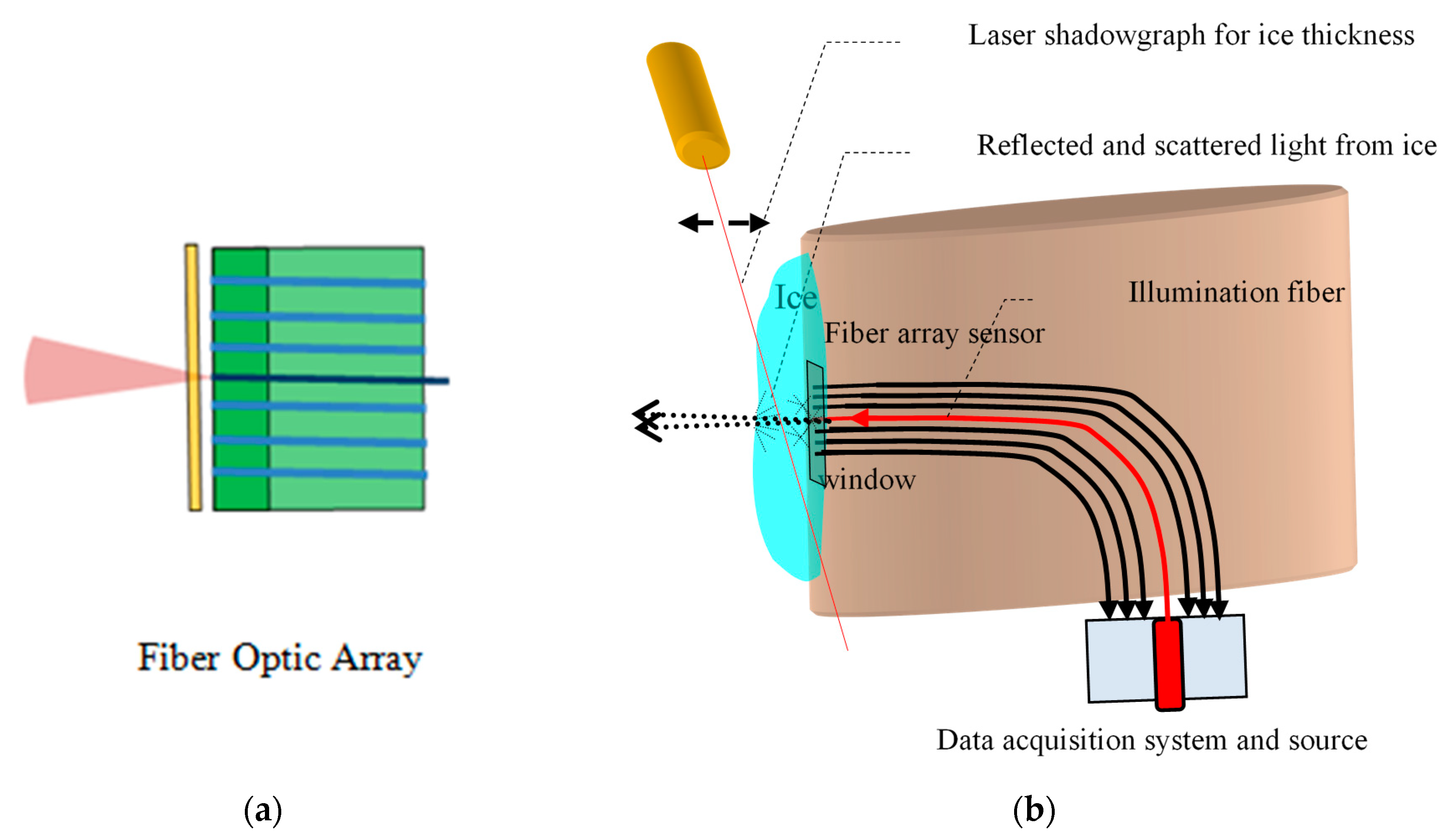
Previously, we have reported an alternative method for direct ice detection based on optical diffusion which measures, in real time, the thickness and type of ice accreted on the wings of aircraft using a fused-silica fiber optical sensor array [
12]. A schematic diagram of the ice sensor and its layout in the icing tunnel is shown in
Figure 15a,b.
In principle, the method relies on illuminating and detecting the light from the accreting ice on the leading edge of the airfoil. Depending on the freezing rate of water, gases dissolved in the super-cooled droplets may or may not escape, forming micro-cracks and micro-bubbles in the ice volume. The density of these discontinuities varies, giving ice its optical characteristics, attributed primarily to Mie scattering [
22].
The fiber array senor, used in the previous work [
12], consists of six multimode flat polished detection signal-fibers, arranged in sets of three, on either side of a central seventh source-fiber with a 2 mm pitch. All the fibers had a NA of 0.1 and the illumination fiber coupled the light from a Laser Diode (LD) emitting at 650 nm (
Figure 15a). Light from the illumination fiber is partially reflected and partially backscattered from the surface and ice volume respectively. The diffuse light is coupled to the signal fibers and transmitted to a set of photodiodes, one for each fiber. The fiber array sensor was located on the stagnation line, of a zero-lift wing, placed vertically in an icing tunnel. All tests were conducted with airspeed of about 150 Knots and temperatures ranging from −5 to −25°C with LWC of 0.5 to 2 gm/m
3. The optical intensity was recorded as a function ice thickness, measured by a shadowgraph technique using a perpendicular laser beam, which traced the front edge on the ice (
Figure 15b).
Depending on the ambient conditions, the accreting ice takes different shapes and forms influenced by the aerodynamics of the airfoil, which generates a local temperature gradient spike over the wing, due to the adiabatic expansion of the air passing over it. A key parameter, which determines the optical characteristics of ice, is the freezing fraction (FF), defined as the ratio of ice that freezes directly on impact to that which remains liquid and freezes behind the impact area [
20,
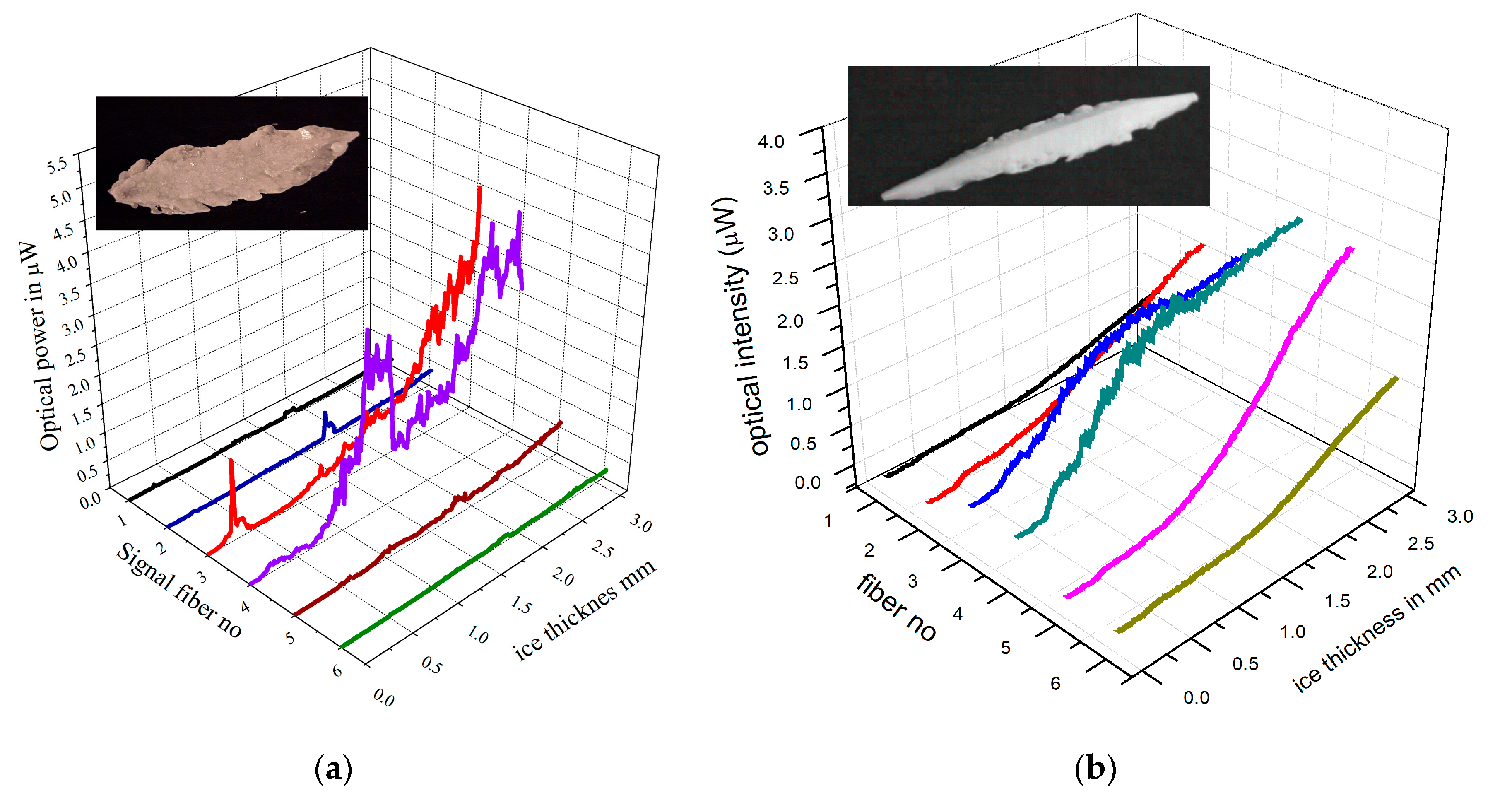
22]. The values of the FF range from zero, for water remaining liquid, to one when all water freezes on impact. The local FF determines the type of ice accreted which can either be clear glazed ice for FF close to 0, opaque rime ice for FF close to 1, or mixed phase ice, with varied transparency, and FF with values between 0 and 1. Typical measurement for glazed and rime ice are shown in
Figure 16a,b, respectively, were the optical intensity is shown as a function of ice thickness for the six, low NA flat-polished signal fibers. In these graphs, the illumination fiber is in between fiber 3 and 4. The maximum detected ice thickness was restricted to about of 3 mm, which is considered a safe threshold for activating the ice protection systems.
In glazed ice (−5 to −10 °C), reflected light from the surface of the ice dominates and signals from the central fibers 3, 4 increase rapidly up to an ice thickness of 3 mm, and exhibit acute intensity spikes. The origin of these intensity spikes is primarily due to transient ice micro-crystals, formed on the surface of the thin transparent ice which can be detected by the inner fibers, being closest to the illumination fiber (
Figure 16a). Conversely, the signals from the outer fibers 1, 2, 5, 6, rise slower with ice thickness, exhibiting overall lower intensities but are “smoother” as they detect predominantly diffuse reflections and scattered light due to the greater distances from the source fiber (
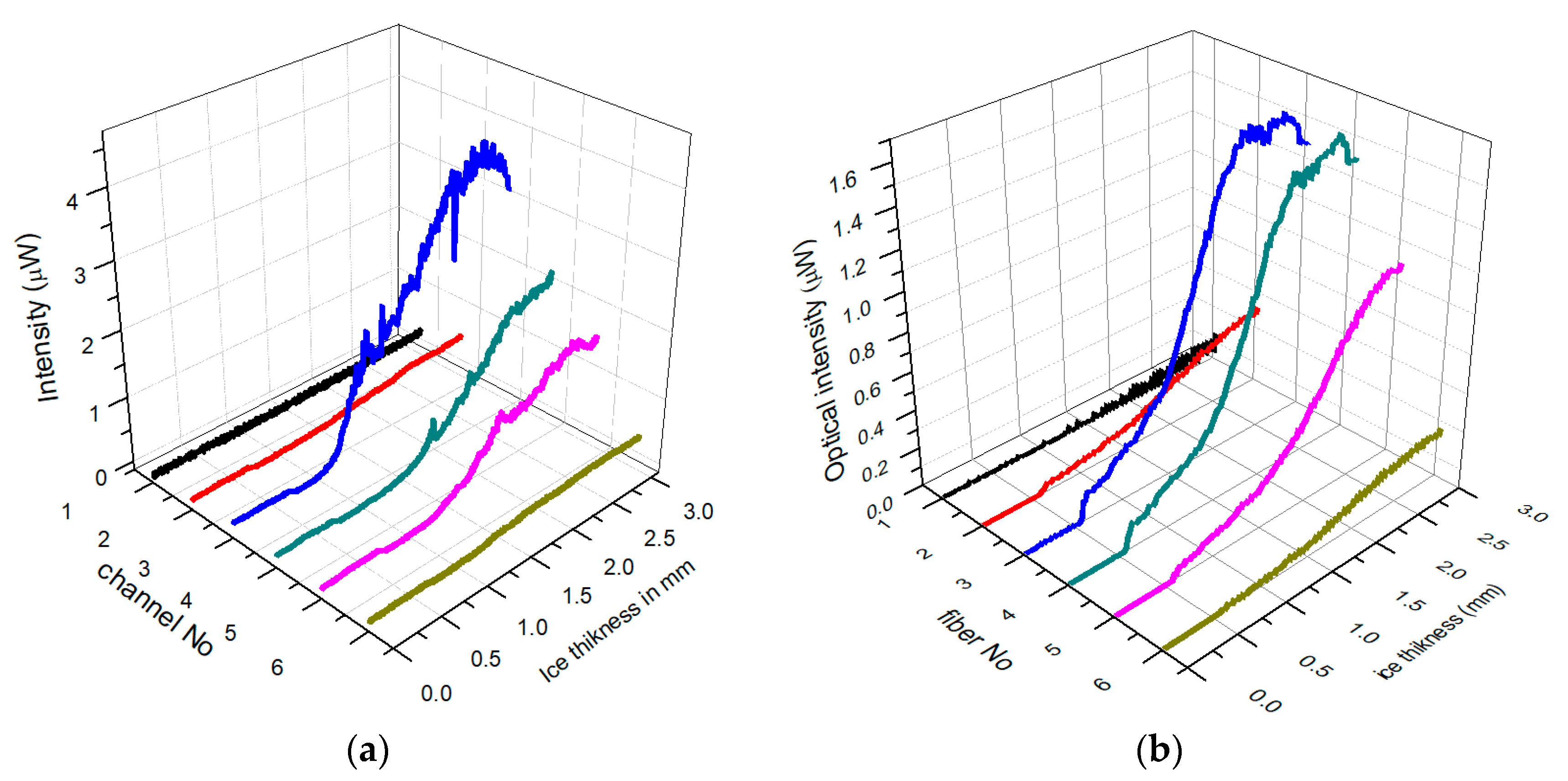
Figure 16a). Similarly, in rime ice (−20 to −25 °C), scattered light dominates, and the intensity distributions are much smoother (
Figure 16b) and lack the intensity peaks seen in glazed ice. In rime ice however, backscattering is the dominant mechanism, as reflected light from surface diffuses in the opaque ice, leading to much smoother signals with virtually no spikes (
Figure 16b).
Another interesting point is that for a low NA fibers-array sensor in glazed ice, the backscattered light is near constant for a particular ice thickness, while the strong transient reflections, near the fiber facet will momentarily contribute a much higher percentage of the detectable power, thus distorting detectible signals. Conversely, if the acceptance angel is increased, light from a much wider “field of view” will be detected, so transient events will represent a lower percentage of the detectable signal, thus averaging out their influence on the signals. Similarly, if the accreting ice is illuminated by a wider beam profile, the overall near field intensity is reduced, thus also reducing the transient reflections. Therefore, this effect can be achieved by using high-NA, MM-POF tapers, both for illumination and detection, utilizing the cutback method as described above.
By retaining the same fiber-array sensor architecture shown in
Figure 16a and replacing the polished fibers with MM POF cleaved tapers, the detection efficiency of the ice sensor can be considerably improved by enchasing the overall NA to about 0.85, with acceptance angles ranging from 120
° to 140
°. Typical results for large NA array sensor are shown in
Figure 17a for glazed ice and
Figure 17b for rime ice.
Similar intensity patens were obtained with the low NA, polished fiber optic array-sensor (
Figure 16a,b) and the POF fibers tapers array sensor (
Figure 17a,b). However, the intensity distributions of glazed ice are much smoother due to the wider illumination of the ice volume and the effective averaging effect of the wider NA of the detection fibers. The elimination of the intensity spikes improves the signal to noise ratio and therefore, significantly improves the detection of ice buildup rate on the leading edge of the wings.

