Abstract
The existing lens correction methods deal with the distortion correction by one or more specific image distortion models. However, distortion determination may fail when an unsuitable model is used. So, methods based on the distortion model would have some drawbacks. A model-free lens distortion correction based on the phase analysis of fringe-patterns is proposed in this paper. Firstly, the mathematical relationship of the distortion displacement and the modulated phase of the sinusoidal fringe-pattern are established in theory. By the phase demodulation analysis of the fringe-pattern, the distortion displacement map can be determined point by point for the whole distorted image. So, the image correction is achieved according to the distortion displacement map by a model-free approach. Furthermore, the distortion center, which is important in obtaining an optimal result, is measured by the instantaneous frequency distribution according to the character of distortion automatically. Numerical simulation and experiments performed by a wide-angle lens are carried out to validate the method.
1. Introduction
Camera lenses suffer from optical aberration; thus, the nonlinear distortion would be introduced into the captured image, especially for the lens with large field of view (FOV). Therefore, distortion correction is a significant problem in the analysis of digital images. The accurate distortion correction of lens is especially crucial for any computer vision task [1,2,3,4] that involves quantitative measurements in the geometric position determination, dimensional measurement, image recognition, and so on. Existing methods for distortion correction can be divided into two main categories: traditional vision measurement methods and learning-based methods.
For the traditional vision measurement methods, it falls into the following main types. One relies on a known measuring pattern [5,6,7], including straight lines, vanishing points, and a planar pattern. It estimates the parameters of the un-distortion function by a known pattern to achieve correction. It is simple and effective, but the distortion center in nonlinear optimization would lead to instabilities [8]. The second is the multiple view correction method [9,10,11], which utilizes the correspondences between points in different images to measure lens distortion parameters. It achieves auto-correction without any special pattern but requires a set of images captured from different views. The third is the plumb-line method [12,13,14,15], which makes the distortion parameter estimation by some distorted circular arcs. Accurate circular arcs detection is a very important aspect for the robustness and flexibility of this kind of method. Human supervision and some robust algorithms for circular arcs detection are developed. All the above-mentioned methods rely on some specific distortion models, such as the commonly used even-order polynomial model [16] proposed by Brown, division model [17] proposed by Fitzgibbon, and fisheye lens model [18]. The whole image achieves distortion correction by employing several characteristic points or lines for the analysis to find out the distortion parameters. It would have poor generalization abilities to other distortion models. Furthermore, it should be noted that all these distortion models achieve ideal circular symmetry.
For the learning-based methods, it can be divided into two kinds. The first one is the parameter-based method [19,20,21], which estimates the distortion parameters by using convolutional neural networks (CNNs) in terms of the single parameter division model or fisheye lens model. It would provide more accurate distortion parameters estimation. However, the networks are still trained by a synthesized distorted image dataset derived from some specific distortion models, which causes inferior results for other types of distortion models. Recently, some distortion correction methods demanding no specific distortion models by deep learning have been proposed. Liao et al. [22] introduced model-free distortion rectification by introducing a distortion distribution map. Li et al. [23] proposed bind geometric distortion correction by using the displacement field between distorted images and corrected images. For these methods, there are different types of distortion models involved into the synthesized distorted image dataset for training, and the distortion distribution map or displacement field are obtained according to these distortion models. It means that the distortion correction is still built on some distortion models, and the employed distortion models are circular symmetry. However, none of the existing mathematical distortion models can work well for all the real lenses with fabrication artifacts.
In addition, there are some model-free distortion correction methods. Munji [24] and Tecklenburg et al. [25] proposed a correction model based on finite elements. The remaining errors in the sensor space can be corrected by interpolation with the finite element. However, the interpolation effect will be reduced when the measured image points are not enough. Grompone von Gioi et al. [26] designed a model-free distortion correction method. It involves great computation and is time consuming, because the optimization algorithm and loop validation are used for high precision.
Fringe-pattern phase analysis [27,28,29], due to its advantage of highly automated full-field analysis, is widely used in various optical measurement technologies, such as interferometry, digital holography, moire fringe measurement, and so on. It is also used for lens distortion determination. Bräuer-Burchardt et al. [30] achieved lens distortion correction by Phasogrammetry. The experiment system and image processing are a bit complicated because both the projector lens distortion and camera lens distortion are involved. Li et al. [31] eliminated the projector lens distortion by employing the Levenberg–Marquardt algorithm for improving the measurement accuracy of fringe projection profilometry, where the lens distortion is described by a polynomial distortion model. We employed the phase analysis of one-dimensional measuring fringe-pattern and polynomial fitting for simple lens distortion elimination by assuming that the distortion is ideal circular symmetry [32].
In this paper, a model-free lens distortion correction based on the phase analysis of a fringe-pattern is proposed. Unlike the method in [32], the proposed method does not rely on circular symmetry assumption. In order to avoid using the distortion model and circular symmetry assumption, the proposed method uses two sets of directional orthogonal fringe patterns to obtain the distortion displacement of all points in the distorted image. Moreover, considering that the distortion center may be displaced from the image center by many factors, such as an offset of the lens center from the sensor center of the camera, a slight tilt of the sensor plane with respect to the lens, a misalignment of the individual components of a compound lens, and so on, the distortion center should be measured in accordance with specific conditions instead of being assumed as the image center directly. For the proposed method, the distortion center is measured by the instantaneous frequency distribution according to the character of distortion automatically. The theoretical description of distortion measurement based on the phase analysis of the sinusoidal fringe-pattern is introduced. The numerical simulation results and experimental results show the validity and advantages of the proposed method.
2. Principle of Model-Free Lens Distortion Correction Method
2.1. Lens Distortion
A simple grid chart of the negative (barrel) distortion, as shown in Figure 1, is employed to present the theoretical description of lens distortion simply and clearly. The blue lines and the red lines are corresponding to the lines before and after distortion, respectively. It is easy to find that the undistorted point comes to the distorted point after distortion. According to the geometry shown in Figure 1, is the distortion displacement according to the distorted point with for the barrel distortion and for the pincushion distortion. So, the point should be corrected to the point , which satisfies:
with and . For image distortion correction, the most important thing is to decide the distortion displacement , i.e., and , at each point. Symbols denotation is given in nomenclature, as shown in Table 1.
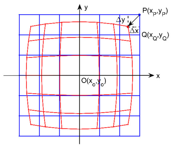
Figure 1.
Distortion schematic diagram for the negative (barrel) distortion, where the blue and red lines are corresponding to the fringe-pattern stripes before and after distortion, respectively.

Table 1.
Nomenclature.
2.2. Phase Analysis of Fringe-Pattern Measuring Template
Two sets of sinusoidal fringe-patterns parallel to the y-axis and x-axis of the display coordinate system, i.e., the longitudinal and transverse fringe-patterns, are employed as measuring templates for phase demodulation analysis to obtain the distortion displacement and , respectively. Figure 2 shows the sinusoidal fringe-patterns before and after barrel distortion, respectively. The undistorted longitudinal and transverse fringe-patterns are expressed as:
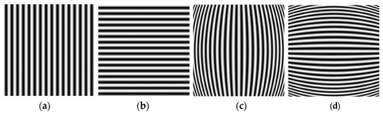
Figure 2.
Sinusoidal fringe-patterns before and after barrel distortion. (a) Undistorted longitudinal fringe-pattern; (b) Undistorted transverse fringe-pattern; (c) Distorted longitudinal fringe-pattern; (d) Distorted transverse fringe-pattern.
The corresponding distorted fringe-patterns are:
where is the background intensity; is the visibility of the fringe-pattern; and are the fundamental spatial frequency of the longitudinal and transverse sinusoidal fringe-pattern, respectively; and are the modulated phase caused by the lens distortion; and are the initial phase. By the analysis of the fringe-patterns, the modulated phase can be obtained point by point, so the distortion displacement and at each point is decided.
2.2.1. Phase of Distorted Fringe-Pattens
The phase-shifting method [33], providing high precision point-to-point phase retrieval from fringe-patterns due to its best spatial localization merit, is employed for phase demodulation. The intensity distributions of the longitudinal and transverse sinusoidal fringe-patterns after distortion are:
where and are the phase of longitudinal and transverse fringe-pattern, respectively; and . By employing the four-step phase-shifting method, the wrapped phase distribution can be acquired from the distorted fringe-patterns as:
The calculated phase is wrapped in by arctangent calculation. So, the unwrapping algorithm [34] is performed, and the continuous phase distribution of the distorted fringe-pattern is obtained. More number of phase shifts would reduce the distortion of the cosine signal and improve the precision of phase demodulation.
2.2.2. Modulated Phase Calculation by Distortion Center Detection
The modulated phases and , which contain the distortion information, are calculated by subtracting the phase and from and , respectively. So, in order to obtain the modulated phase, the fundamental spatial frequency and should be detected. According to the distortion character, there is no distortion at the distortion center. Therefore, the fundamental spatial frequency of the fringe-pattern is detected at the position of the distortion center. It should be noticed that the distortion center may be significantly displaced from the center of the image by many factors. For the proposed method, the distortion center can be measured by the instantaneous frequency distribution automatically. It is at the position where the minimum instantaneous frequency appears for the barrel distortion and the maximum instantaneous frequency appears for the pincushion distortion. So, we perform the partial derivative operation along the and direction of the phase and to get the instantaneous frequency and respectively as:
By judging the variation trend of instantaneous frequency, the type of distortion could be determined. When the instantaneous frequency increases along the radial direction from the distortion center, it is the barrel distortion. Otherwise, it is the pincushion distortion. Then, by detecting the position of the minimum and along the and direction for the barrel distortion, or the position of the maximum and for the pincushion distortion, the distortion center can be decided as . So, the corresponding fundamental frequencies are determined at as:
According to and , the phase distribution and can be calculated, and the modulated phase can be rewritten as and :
where and are the phase of the longitudinal and transverse sinusoidal fringe-patterns at the distortion center.
2.2.3. Relationship of Modulated Phase and Distortion Displacement
The distortion displacement and are obtained by the modulated phase as:
Therefore, the measurement of the distortion displacement is transferred into the calculation of the modulated phase by the fringe-pattern analysis. In a word, the distortion displacement and can be measured point by point according to the phase demodulation analysis of the distorted sinusoidal fringe-patterns.
2.2.4. Distortion Correction
The inverse mapping method with the bilinear interpolation is employed for the image distortion correction. It should be noticed that the distortion displacement obtained by Equation (9) corresponds to the points on the distorted fringe-pattern. So, we recalculate the distortion displacement and , which correspond to the points on the corrected fringe-pattern. Firstly, we establish the discrete numerical correspondences of the new distortion displacement and with the points on the corrected fringe-pattern. It should be noticed that the calculated coordinate value of the points on the corrected fringe-pattern may not be integer. So, we calculate the distortion displacement and by performing the bicubic interpolation algorithm, where is the integer coordinate value of the corrected point. Therefore, the distribution of the distortion displacement corresponding to the points on the corrected fringe-pattern is decided, and the image distortion correction can be achieved by adopting the inverse mapping method directly by:
where is the corresponding distorted point. Finally, the bilinear interpolation algorithm is employed for the image interpolation not only because of the simple and convenient calculation process but also due to its ability of overcoming the problem of gray-scale discontinuity.
3. Numerical Simulation
Numerical simulation is performed to verify the validity of the method we introduced. Firstly, two sets of longitudinal and transverse sinusoidal fringe-patterns of pixels with a phase shift of are employed as measuring patterns. The spatial period of the undistorted fringe-pattern is 16 pixels. Then, the single parameter division model [17] with distortion parameter , given by Equation (11), is employed to generate the barrel distorted fringe-patterns.
where and are the Euclidean distance of the distorted and undistorted point to the distortion center, respectively. Moreover, the distortion center is shifted away from the image center to . Figure 3 shows the corresponding distorted fringe-patterns, respectively. It should be noticed that the proposed method is model-free. The single parameter division model employed here, which can be replaced by any other distortion model, is just to generate a simulated distorted image.
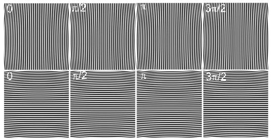
Figure 3.
Simulated distorted fringe-patterns of size pixels by a single parameter division model with a distortion parameter and distortion center . The longitudinal fringe-patterns with a phase shift of are at the first row and the transverse fringe-patterns with a phase shift of are at the second row.
The analysis process and the corresponding results can be described as follows.
Step 1: Employ the four-step phase-shifting method for the phase demodulation and perform the unwrapping algorithm to obtain the phase distribution of the distorted longitudinal and transverse fringe-patterns. Figure 4a,b are the corresponding wrapped phase.
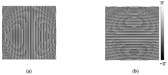
Figure 4.
Wrapped phase. (a) Wrapped phase of distorted longitudinal fringe-pattern; (b) Wrapped phase of a distorted transverse fringe-pattern transverse.
Step 2: Calculate the instantaneous frequency and . It is determined as barrel distortion because the instantaneous frequency increases along the radial direction from the distortion center. By detecting the minimum along the direction, we can find that the distortion center is at the 273th column. Similarly, by detecting the minimum along the direction, we can find that the distortion center is at the 289th row. So, the distortion center is at . Figure 5a,b and , where the red dotted lines are at the 289th row and 273th column, respectively. Figure 5c,d are the corresponding distribution of at the 289th row and at the 273th column, respectively. The fundamental frequency is and the phase and at the distortion center are obtained.
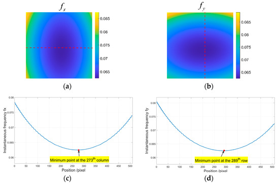
Figure 5.
Instantaneous frequency. (a) ; (b) ; (c) at the 289th row with the minimum point at the 173th column; (d) at the 273th column with the minimum point at the 289th row.
Step3: Modulated phase calculation. According to Equation (8), the modulated phase and are obtained as shown in Figure 6a,b. So, the distortion displacement and are obtained point by point according to Equation (9), as shown in Figure 6c,d. The distortion displacement can be obtained by Equation (1), and the maximum error of is 0.24 pixels. In order to further validate the proposed method, distortion parameter estimation according to the single parameter division model is performed. The estimated distortion parameter is with the relative error of 0.8%.
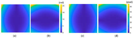
Figure 6.
Modulated phase and distortion displacement. (a) ; (b) ; (c) ; (d) .
Step4: Distortion displacement map calculation. We establish the discrete numerical correspondences of the new distortion displacement and with the points on the corrected fringe-pattern. Table 2 shows some of the distortion displacement of the points on the distorted fringe-pattern and the corresponding points on the corrected fringe-pattern. We find that the calculated coordinates of the points on the corrected fringe-pattern are not integers. So, we calculate the distortion displacement and by performing the bicubic interpolation algorithm, where is the integer coordinate value of the corrected point.
Table 2.
Some calculated distortion displacement (pixel).
Step5: According to the distortion displacement map, image distortion correction can be performed by employing the inverse mapping with the bilinear interpolation directly.
A numerical simulation of the distorted checkerboard is performed. Figure 7a shows the distorted checkerboard image with the same distortion parameter of and distortion center . Figure 7b is the corrected result by the proposed method, where the red points represent the corners. Figure 8 is the corresponding corners image, where the red asterisks represent the corners of the distorted checkerboard image and the blue points represent the corners of the corrected checkerboard image. The distortion displacement at the left top point is pixel. The curvature radius of the red line formed by the left points on the distorted checkerboard image is pixels, and that of the blue line corresponding to the corrected checkerboard image is pixels. It means that the circular arc is corrected to be straight.
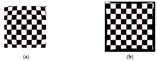
Figure 7.
Analyzed results of checkerboard image, where the red points represent the corners. (a) Distorted checkerboard image with distortion parameter and distortion center ; (b) Corrected image.
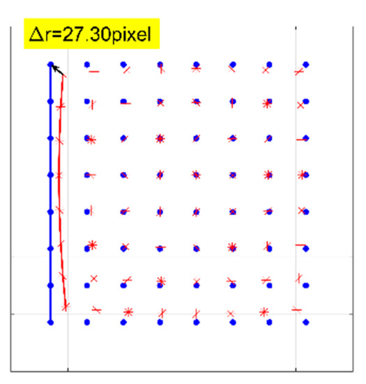
Figure 8.
Corners image with the red asterisks representing the corners of the distorted checkerboard image and the blue points representing the corners of the corrected checkerboard image. The curvature radius of the red line is pixels, and that of the blue line is pixels.
4. Experiment and Results
An experimental setup shown in Figure 9 is employed to perform distortion correction of a wide-angle lens. A flat-panel liquid crystal display (LCD) is used to display two sets of longitudinal and transverse sinusoidal fringe-patterns with phase shift of . The images of these fringe-patterns are captured by a charge-couple device (CCD) camera with a wide-angle lens. The LCD plane can be regarded as an ideal plane, and the optical axis of the camera is perpendicular to the LCD plane. The distorted fringe-patterns captured by the camera are shown in Figure 10. Figure 11a,b show the intensity distributions of the central row and column of the longitudinal and transverse fringe-patterns with a phase shift of , respectively.
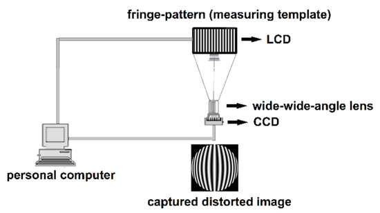
Figure 9.
Experimental setup. Liquid crystal display (LCD): FunTV D49Y; wide-angle lens: Theia MY125M, FOV1370; charge-couple device (CCD) camera: PointGrey CM3-U3-50S5M-CS, 2048 × 2448 pixels, 3.45 μm pixel size.
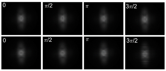
Figure 10.
Distorted fringe-patterns of size 2048 × 2448 pixels. The longitudinal fringe-patterns with a phase shift of are in the first row and the transverse with a phase shift of are in the second row.
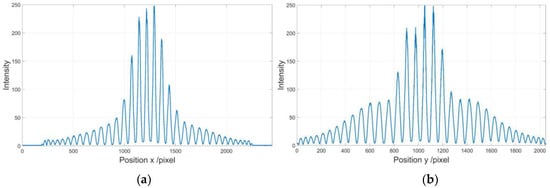
Figure 11.
Intensity distribution of the distorted fringe-patters. (a) Intensity of the central row of the longitudinal fringe-pattern with a phase shift of ; (b) Intensity of the central column of the transverse fringe-pattern with a phase shift of .
By performing the four-step phase-shifting analysis, the wrapped phases of the distorted longitudinal and transverse fringe-patterns are obtained as shown in Figure 12a,b. It shows that the phase of the distorted fringe-pattern can be demodulated well even when the intensity distribution of the fringe-patterns is low within some areas. The corresponding unwrapped phase can be obtained by performing the unwrapping algorithm. First, we perform the partial derivative operation of the phase of the distorted longitudinal and transverse fringe-pattern to get the instantaneous frequency and , respectively. The type of distortion is determined as barrel distortion for the instantaneous frequency increases along the radial direction. Then, the distortion center is decided at according to the distribution of the instantaneous frequency and . Considering the fluctuation of the analyzed phase caused by the noise in the experiment, we perform numerical linear fitting to calculate the phase of the undistorted fringe-pattern by employing the central 25 points of the phase of the distorted longitudinal and transverse fringe-pattern respectively, instead of performing the calculation by the instantaneous frequency and phase at the distortion center. The points of and are employed for calculation. The fundamental frequencies are . The modulated phase distribution and are obtained as shown in Figure 13a,b respectively. Figure 13c,d show the numerical distortion displacement map and of size pixels. Finally, by employing the inverse mapping with the bilinear interpolation, the image distortion correction can be achieved.
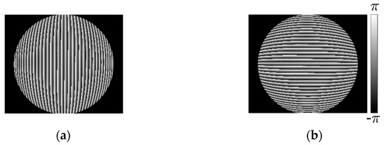
Figure 12.
Wrapped phase. (a) Wrapped phase of distorted longitudinal fringe-pattern; (b) Wrapped phase of distorted transverse fringe-pattern transverse.
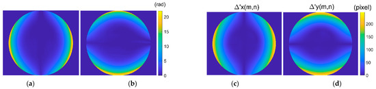
Figure 13.
Modulated phase and distortion displacement map. (a) of size pixels; (b) of size pixels; (c) of size pixels; (d) of size pixels.
Figure 14 shows the experiment of checkerboard images, where Figure 14a is the distorted image and Figure 14b is the corrected image with the red points representing the corners by the proposed model-free method. Figure 15 is the corresponding corners image, where the red asterisks represent the corners of the distorted checkerboard image and the blue points represent the corners of the corrected checkerboard image. The distortion displacement at the left top point is pixels. The curvature radius of the red line formed by the left points on the distorted checkerboard image is pixels, and that of the blue line corresponding to the corrected checkerboard image is pixels. The larger the curvature radius, the closer the curve is to the straight line, i.e., the better the correction effect.
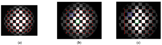
Figure 14.
Experimental results of checkerboard images. (a) Distorted checkerboard image of size pixels; (b) Corrected image of size pixels with the red points representing the corners by the proposed model-free method. The pixel count of the square within the central green rectangular region is 49,033 pixels, and that of the square within the external blue rectangular region is 48,460 pixels. (c) Corrected image by plumb-line method. The curvature radius of the red line is pixels. The pixel count of the square within the central green rectangular region is pixels, and that of the square within the external blue rectangular region is 57,490 pixels.
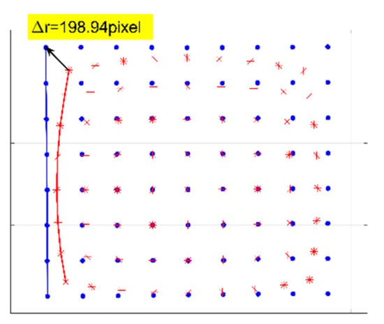
Figure 15.
Corners image with the red asterisks representing the corners of the distorted checkerboard image and the blue points representing the corners of the corrected checkerboard image corresponding to those shown in Figure 14a,b. The curvature radius of the red line is pixels, and that of the blue line is pixels.
Firstly, we perform distortion correction by the plumb-line method with a single parameter division model [12] for comparison. The red line shown in Figure 15 is employed for the estimation of the distortion parameter. The estimated is . According to Equation (11), the distortion displacement can be numerically calculated. The corrected image is shown in Figure 14c, where the red points represent the corners. The curvature radius of the red line is pixels, compared with the corresponding curvature radius of pixels by the proposed method. Moreover, the square within the central region is not the same size as the square at the external region in the corrected image as shown in Figure 14c. We select two white squares at the central and external region to show the difference. The pixel count of the square within the central green rectangular region is 46,988 pixels compared that of the square within the external blue rectangular region being 57,490 pixels. By the proposed method, the pixel counts of these two corresponding squares are 49,033 and 48,460 pixels as shown in Figure 14b. It means that the estimated distortion lambda of the single parameter division model by this characteristic circular arc does not fit for the whole image correction.
On the other hand, in order to make comparison with the method employing some distortion models, we employ the method in [32] for distortion displacement detection. We take the distortion center point as the origin of the coordinate and perform the numerical curve fitting according to the discrete distortion displacement from the 1224th to the 2556th point at the 1008th row by three different distortion models, which are an even-order polynomial model with one and two distortion parameters and single parameter division model. The even-order polynomial model [16] is described as:
Figure 16 shows the curve fitting results, where the black line is the analyzed radial distortion displacement, the green line is the curve fitting result of the even-order polynomial model with , the red line is that of the even-order polynomial model with , and the blue line is that of the single parameter division model with . We can find that the fitting result by the even-order polynomial model with two distortion parameters is better.
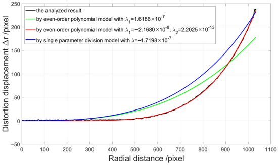
Figure 16.
Radial distortion displacement and curve fitting results.
Figure 17 shows the corresponding correction results of the checkerboard image respectively, where Figure 17a,b are by the even-order polynomial model with one and two distortion parameters, respectively, and Figure 17c is by the single parameter division model. The curvature radius of the line formed by the left points on the corrected checkerboard image is pixels, pixels, and pixels respectively compared with the corresponding curvature radius of pixels by the proposed method. The pixel counts of the above-mentioned squares at the central and external regions in the corrected image by the even-order polynomial model with two distortion parameters are 48,094 and 48,694 pixels, as shown in Figure 17b. We can find that the curve fitting results rely on the distortion model greatly. Distortion determination may fail using an unsuitable model or by estimation of too few distortion parameters. However, the more distortion parameters there are, the more complicated the solution of the reverse process.
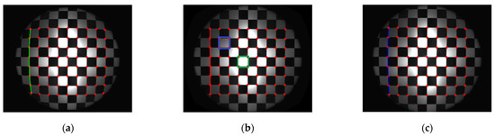
Figure 17.
Experimental results of checkerboard images. (a) Corrected image by a one-parameter even-order polynomial model with a green line curvature radius of pixels. (b) Corrected image by a two-parameter even-order polynomial model with a red line curvature radius of pixels. The pixel count of the square within the central green rectangular region is 48,094 pixels, and that of the square within the external blue rectangular region is 48,694 pixels. (c) Corrected image by a single parameter division model with a blue line curvature radius of pixels.
Furthermore, the indoor and outdoor scenes are also employed for the experiment to show the practicality of the proposed method. Figure 18 and Figure 19 show the corresponding distorted and corrected image, respectively. The experimental results show that the distorted images achieve distortion correction effectively by the proposed model-free method.
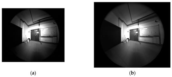
Figure 18.
Experimental results of the indoor scene. (a) Distorted image of size 2048 × 2448 pixels; (b) Corrected image of size 2496 × 2984 pixels.
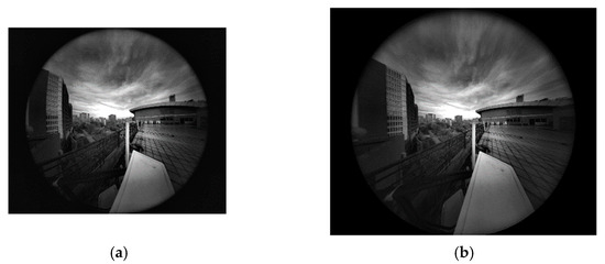
Figure 19.
Experimental results of the outdoor scene. (a) Distorted image of size pixels; (b) Corrected image of size pixels.
5. Discussion
Experimental correction results of the checkerboard image by different methods are given for the comparison with the proposed model-free correction method. The original straight line is distorted into a circular arc with a curvature radius of pixels, as shown in Figure 15. By the plumb-line method with the single parameter division model, the phase analysis method by the even-order polynomial model with one and two distortion parameters and the single parameter division model, and the proposed model-free method, the curvature radiuses of the corresponding corrected lines on the corrected checkerboard images are , ,,, and pixels, respectively. The circular arc is corrected to be straighter by the proposed method. It means that the proposed method provides a superior result, and it shows that distortion determination may fail using an unsuitable model firstly. Moreover, from the comparison of the curvature radius of the corresponding corrected lines, it seems that the corrected result of the plumb-line method is better than that by the phase analysis method by the even-order polynomial model with two distortion parameters. The reason for this is that the distortion parameter estimation by the plumb-line method is performed by the distorted circular arc at this position. However, for the corrected checkerboard image by the plumb-line method, the square within the central region of size 46,988 pixels is not the same as the square at the external region of size 57,490 pixels. It means that the estimated distortion parameter does not fit for the whole image correction. Therefore, according to the analysis result, we should take more characteristic points and lines or some other more complicated algorithm or distortion models into account. However, the more distortion parameters there are, the more complicated the solution of the reverse process. For the proposed model-free method, all points of the distorted fringe-pattern are employed for the establishment of the distortion displacement map, which demands none of the distortion model. So, the image achieve distortion correction point by point with a more effective and satisfactory result.
In the experiment of distortion displacement measurement, the errors caused by the nonideal LCD plane and imperfect perpendicular arrangement of the optical axis of camera and the LCD plane should be considered.
6. Conclusions
In this paper, a model-free lens distortion correction method based on the distortion displacement map by the phase analysis of fringe-patterns is proposed. For the image distortion correction, the most important thing is to decide the distortion displacement. So, the mathematical relationship of the distortion displacement and the modulated phase of the fringe-pattern is established in theory firstly. Then, two sets of longitudinal and transverse fringe-patterns are employed for phase demodulation analysis to obtain the distortion displacement and respectively by the phase-shifting method. The distortion displacement map can be determined point by point for the whole distorted image to achieve distortion correction. It would be effective even when the circular symmetry condition is not satisfied. Moreover, it detects the radial distortion type and the distortion center automatically according to the instantaneous frequency, which is important in obtaining optimal result. The correction results of the numerical simulation, experiments, and comparison show the effectiveness and superiority of the proposed method.
There are some prospects of our further works. Firstly, the relationship of the modulated phase and the distortion displacement described by the proposed method would still hold for the mix distortion with the radial and tangential type. However, if the tangential distortion is severe, the distortion center would not be the corresponding position where the minimum or maximum instantaneous frequency appears. So, how to decide the distortion center automatically in this case should be considered. Secondly, the optimal frequency of measuring fringe-patterns for accurate modulated phase analysis should be considered. Thirdly, the application of the proposed method should be implemented.
Author Contributions
Conceptualization, J.Z. and J.W.; software, J.W., S.M. and P.Q.; investigation, W.Z.; writing, J.W. and J.Z.; supervision, J.Z. All authors have read and agreed to the published version of the manuscript.
Funding
This research was funded by the National Natural Science Foundation of China, grant number 61875074 and 61971201; the Natural Science Foundation of Guangdong Province, grant number 2018A030313912; the Open Fund of the Guangdong Provincial Key Laboratory of Optical Fiber Sensing and Communications (Jinan University).
Institutional Review Board Statement
Not applicable.
Informed Consent Statement
Not applicable.
Data Availability Statement
Data sharing not applicable.
Conflicts of Interest
The authors declare no conflict of interest.
References
- Collins, T.; Bartoli, A. Planar structure-from-motion with affine camera models: Closed-form solutions, ambiguities and degeneracy analysis. IEEE Trans. Pattern Anal. Mach. Intell. 2017, 39, 1237–1255. [Google Scholar] [CrossRef]
- Guan, H.; Smith, W.A.P. Structure-from-motion in spherical video using the von Mises-Fisher distribution. IEEE Trans. Image Process. 2017, 26, 711–723. [Google Scholar] [CrossRef]
- Herrera, J.L.; Del-Blanco, C.R.; Garcia, N. Automatic depth extraction from 2D images using a cluster-based learning framework. IEEE Trans. Image Process. 2018, 27, 3288–3299. [Google Scholar] [CrossRef]
- Wang, Y.; Deng, W. Generative model with coordinate metric learning for object recognition based on 3D models. IEEE Trans. Image Process. 2018, 27, 5813–5826. [Google Scholar] [CrossRef]
- Devernay, F.; Faugeras, O. Straight lines have to be straight. Mach. Vis. Appl. 2001, 13, 14–24. [Google Scholar] [CrossRef]
- Ahmed, M.; Farag, A. Non-metric calibration of camera lens distortion: Differential methods and robust estimation. IEEE Trans. Image Process. 2005, 14, 1215–1230. [Google Scholar] [CrossRef]
- Cai, B.; Wang, Y.; Wu, J.; Wang, M.; Li, F.; Ma, M.; Chen, X.; Wang, K. An effective method for camera calibration in defocus scene with circular gratings. Opt. Lasers Eng. 2019, 114, 44–49. [Google Scholar] [CrossRef]
- Swaminathan, R.; Nayar, S. Non metric calibration of wide-angle lenses and polycameras. IEEE Trans. Pattern Anal. Mach. Intell. 2000, 22, 1172–1178. [Google Scholar] [CrossRef]
- Hartley, R.; Kang, S.B. Parameter-free radial distortion correction with center of distortion estimation. IEEE Trans. Pattern Anal. Mach. Intell. 2007, 29, 1309–1321. [Google Scholar] [CrossRef]
- Kukelova, Z.; Pajdla, T. A minimal solution to radial distortion autocalibration. IEEE Trans. Pattern Anal. Mach. Intell. 2011, 33, 2410–2422. [Google Scholar] [CrossRef]
- Gao, Y.; Lin, C.; Zhao, Y.; Wang, X.; Wei, S.; Huang, Q. 3-D surround view for advanced driver assistance systems. IEEE Trans. Pattern Anal. Mach. Intell. 2018, 19, 320–328. [Google Scholar] [CrossRef]
- Bukhari, F.; Dailey, M.N. Automatic radial distortion estimation from a single image. J. Math. Imaging Vis. 2013, 45, 31–45. [Google Scholar] [CrossRef]
- Alemán-Flores, M.; Alvarez, L.; Gómez, L.; Santana-Cedrés, D. Automatic lens distortion correction using one-parameter division models. Image Process. Line 2014, 4, 327–343. [Google Scholar] [CrossRef]
- Santana-Cedrés, D.; Gómez, L.; Alemán-Flores, M. An iterative optimization algorithm for lens distortion correction using two-parameter models. Image Process. Line 2016, 5, 326–364. [Google Scholar] [CrossRef]
- Li, L.; Liu, W.; Xing, W. Robust radial distortion correction from a single image. In Proceedings of the 2017 IEEE 15th International Conference on Dependable, Autonomic and Secure Computing, 15th International Conference on Pervasive Intelligence and Computing, 3rd International Conference on Big Data Intelligence and Computing and Cyber Science and Technology Congress(DASC/PiCom/DataCom/CyberSciTech), Orlando, FL, USA, 6–10 November 2017; pp. 766–772. [Google Scholar]
- Brown, D.C. Close-range camera calibration. Photogramm. Eng. 1971, 37, 855–886. [Google Scholar]
- Fitzgibbon, A.W. Simultaneous linear estimation of multiple view geometry and lens distortion. In Proceedings of the 2001 IEEE Computer Society Conference on Computer Vision and Pattern Recognition, CVPR 2001, Kauai, HI, USA, 8–14 December 2001; pp. I125–I132. [Google Scholar]
- Kannala, J.; Brandt, S. A generic camera model and calibration method for conventional, wide-angle, and fish-eye lenses. IEEE Trans. Pattern Anal. Mach. Intell. 2006, 28, 1335–1340. [Google Scholar] [CrossRef]
- Rong, J.; Huang, S.; Shang, Z.; Ying, X. Radial lens distortion correction using convolutional neural networks trained with synthesized images. In Asian Conference on Computer Vision; Springer: Cham, Switzerland, 2016; pp. 35–49. [Google Scholar]
- Yin, X.; Wang, X.; Yu, J.; Zhang, M.; Fua, P.; Tao, D. FishEyeRecNet: A multi-context collaborative deep network for fisheye image rectification. In Proceedings of the European Conference on Computer Vision, Munich, Germany, 8–14 September 2018; pp. 475–490. [Google Scholar]
- Xue, Z.; Xue, N.; Xia, G.; Shen, W. Learning to Calibrate Straight Lines for Fisheye Image Rectification. In Proceedings of the 2019 IEEE/CVF Conference on Computer Vision and Pattern Recognition (CVPR), Long Beach, CA, USA, 15–20 June 2019; pp. 1643–1651. [Google Scholar]
- Liao, K.; Lin, C.; Zhao, Y.; Xu, M. Model-Free Distortion Rectification Framework Bridged by Distortion Distribution Map. IEEE Trans. Image Process. 2020, 29, 3707–3717. [Google Scholar] [CrossRef]
- Li, X.; Zhang, B.; Sander, P.V.; Liao, J. Blind Geometric Distortion Correction on Images through Deep Learning. In Proceedings of the 2019 IEEE/CVF Conference on Computer Vision and Pattern Recognition (CVPR), Long Beach, CA, USA, 15–20 June 2019; pp. 4850–4859. [Google Scholar]
- Munjy, R.A.H. Self-Calibration using the finite element approach. Photogramm. Eng. Remote Sens. 1986, 52, 411–418. [Google Scholar]
- Tecklenburg, W.; Luhmann, T.; Heidi, H. Camera Modelling with Image-variant Parameters and Finite Elements. In Optical 3-D Measurement Techniques V; Wichmann Verlag: Heidelberg, Germany, 2001. [Google Scholar]
- Gioi, R.G.V.; Monasse, P.; Morel, J.M.; Tang, Z. Towards high-precision lens distortion correction. In Proceedings of the International Conference on Image Processing, ICIP 2010, Hong Kong, China, 12–15 September 2010; pp. 4237–4240. [Google Scholar]
- Takeda, M.; Mutoh, K. Fourier transform profilometry for the automatic measurement of 3-D object shapes. Appl. Opt. 1983, 22, 3977–3982. [Google Scholar] [CrossRef]
- Zhong, J.; Weng, J. Phase retrieval of optical fringe patterns from the ridge of a wavelet transform. Opt. Lett. 2005, 30, 2560–2562. [Google Scholar] [CrossRef]
- Weng, J.; Zhong, J.; Hu, C. Digital reconstruction based on angular spectrum diffraction with the ridge of wavelet transform in holographic phase-contrast microscopy. Opt. Express 2008, 16, 21971–21981. [Google Scholar] [CrossRef] [PubMed]
- Braeuer-Burchardt, C. Correcting lens distortion in 3D measuring systems using fringe projection. Proc. SPIE Int. Soc. Opt. Eng. 2005, 5962, 155–165. [Google Scholar]
- Li, K.; Bu, J.; Zhang, D. Lens distortion elimination for improving measurement accuracy of fringe projection profilometry. Opt. Lasers Eng. 2016, 85, 53–64. [Google Scholar] [CrossRef]
- Zhou, W.; Weng, J.; Peng, J.; Zhong, J. Wide-angle lenses distortion calibration using phase demodulation of phase-shifting fringe-patterns. Infrared Laser Eng. 2020, 49, 20200039. [Google Scholar] [CrossRef]
- Zuo, C.; Feng, S.; Huang, L.; Tao, T.; Yin, W.; Chen, Q. Phase shifting algorithms for fringe projection profilometry: A review. Opt. Lasers Eng. 2018, 109, 23–59. [Google Scholar] [CrossRef]
- Ghiglia, D.C.; Pritt, M.D. Two-Dimensional Phase Unwrapping: Theory, Algorithms, and Software; Wiley: Hoboken, NJ, USA, 1998; pp. 181–215. [Google Scholar]
Publisher’s Note: MDPI stays neutral with regard to jurisdictional claims in published maps and institutional affiliations. |
© 2020 by the authors. Licensee MDPI, Basel, Switzerland. This article is an open access article distributed under the terms and conditions of the Creative Commons Attribution (CC BY) license (http://creativecommons.org/licenses/by/4.0/).