Figure 1.
Austenitic steel tube (SUS304H) used in thermal power plant boilers and their modeling; (a) specimen, (b) weld geometry of tube.
Figure 1.
Austenitic steel tube (SUS304H) used in thermal power plant boilers and their modeling; (a) specimen, (b) weld geometry of tube.
Figure 2.
Metal crystal structure of the austenitic steel weld [
27,
28].
Figure 2.
Metal crystal structure of the austenitic steel weld [
27,
28].
Figure 3.
Weld modeling method. (
a) Ogilvy’s model, (
b) classification into domains with electron backscatter diffraction (EBSD) scanning [
31], (
c) classification into six domains with uniform orientation.
Figure 3.
Weld modeling method. (
a) Ogilvy’s model, (
b) classification into domains with electron backscatter diffraction (EBSD) scanning [
31], (
c) classification into six domains with uniform orientation.
Figure 4.
Phased array (PA) probe modeling for simulation; (a) longitudinal 2D linear, (b) transverse.
Figure 4.
Phased array (PA) probe modeling for simulation; (a) longitudinal 2D linear, (b) transverse.
Figure 5.
Beam propagation according to skip distance.
Figure 5.
Beam propagation according to skip distance.
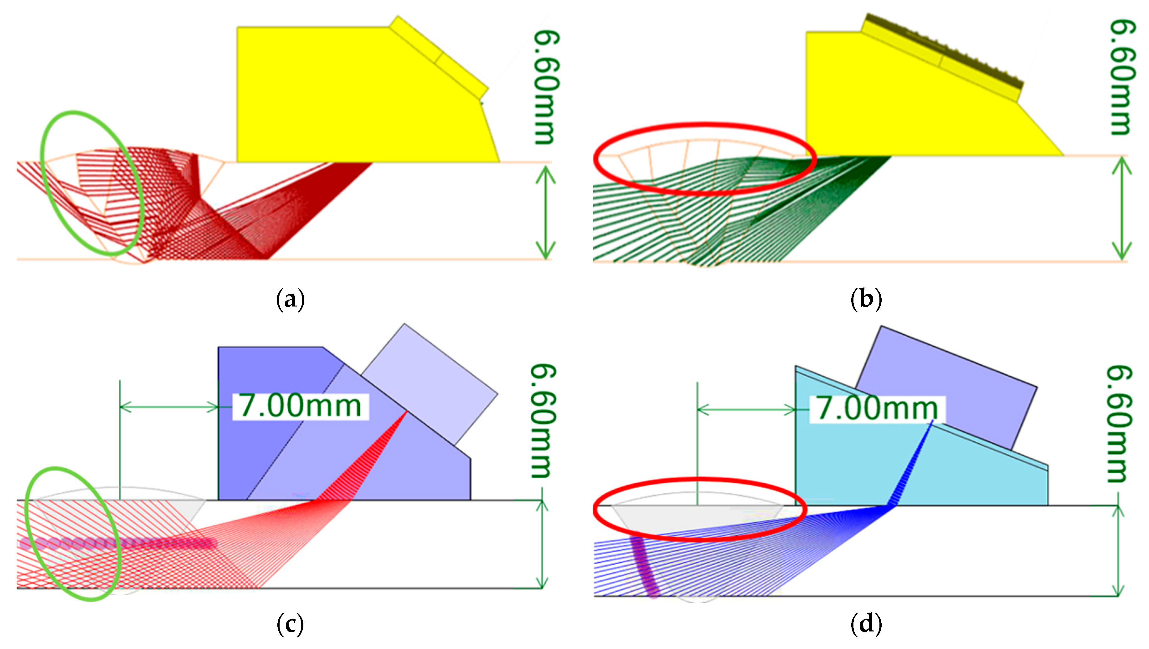
Figure 6.
Beam computation results for transverse waves; at 7.5 MHz (a) isotropic and (b) classification into six domains; at 4 MHz (c) isotropic and (d) classification into six domains.
Figure 6.
Beam computation results for transverse waves; at 7.5 MHz (a) isotropic and (b) classification into six domains; at 4 MHz (c) isotropic and (d) classification into six domains.
Figure 7.
Beam computation results for longitudinal waves at 5 MHz (a) isotropic and (b) classification into six domains.
Figure 7.
Beam computation results for longitudinal waves at 5 MHz (a) isotropic and (b) classification into six domains.
Figure 8.
Scan plan for sectorial beam; classification into six domains (a) transverse wave scan plan and (b) longitudinal wave scan plan, isotropic (c) transverse wave scan plan and (d) longitudinal wave scan plan.
Figure 8.
Scan plan for sectorial beam; classification into six domains (a) transverse wave scan plan and (b) longitudinal wave scan plan, isotropic (c) transverse wave scan plan and (d) longitudinal wave scan plan.
Figure 9.
Specimen for sensitivity calibration and modeling; (a) sensitivity calibration block, (b) modeling for sensitivity calibration.
Figure 9.
Specimen for sensitivity calibration and modeling; (a) sensitivity calibration block, (b) modeling for sensitivity calibration.
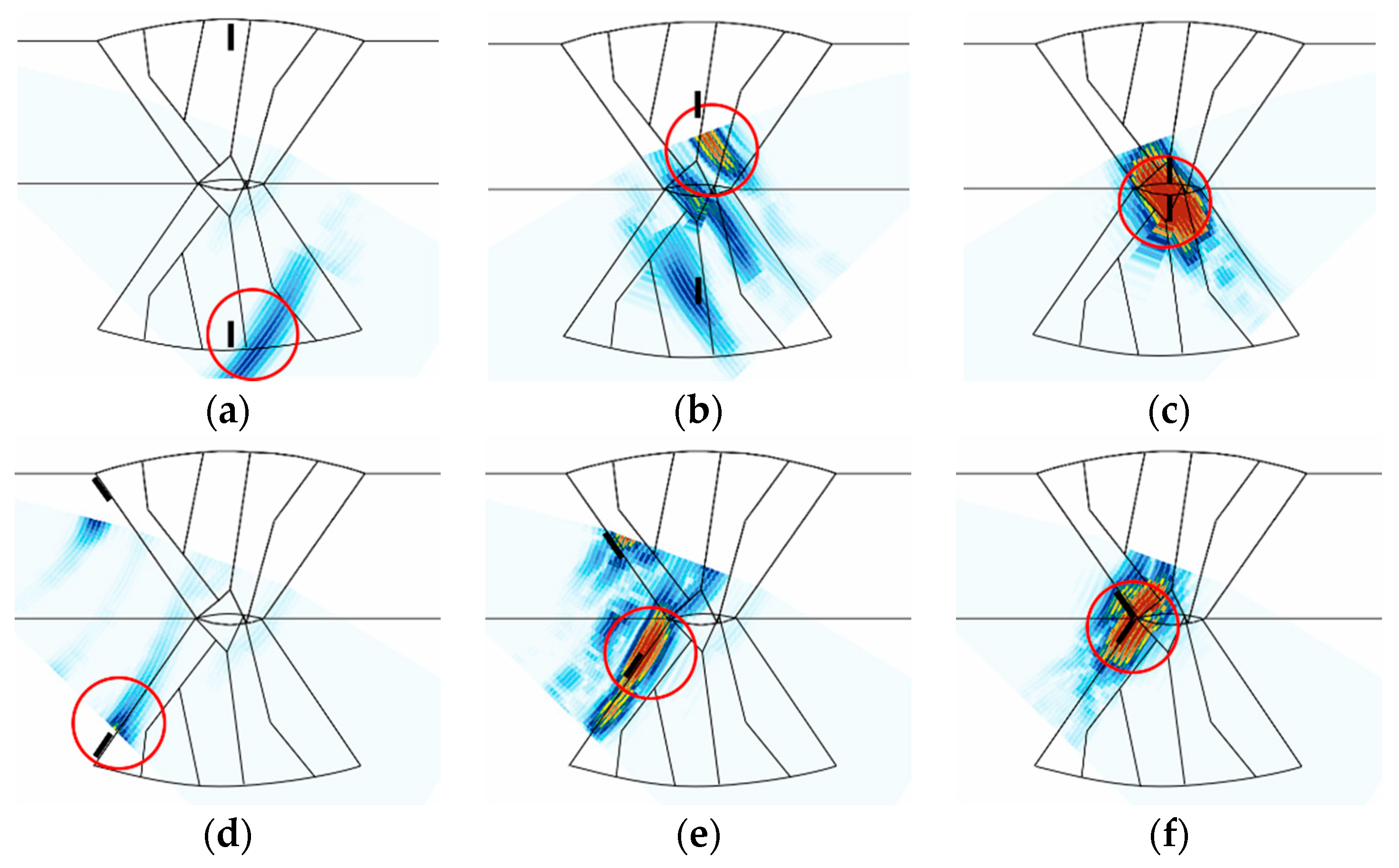
Figure 10.
S-scan results of flaw detection simulation using transverse waves at a frequency of 4 MHz; (a) top crack, (b) middle crack, (c) bottom crack, (d) top LF, (e) middle LF, (f) bottom LF.
Figure 10.
S-scan results of flaw detection simulation using transverse waves at a frequency of 4 MHz; (a) top crack, (b) middle crack, (c) bottom crack, (d) top LF, (e) middle LF, (f) bottom LF.
Figure 11.
S-scan results of flaw detection simulation using transverse waves at a frequency of 7.5 MHz; (a) top crack, (b) middle crack, (c) bottom crack, (d) top LF, (e) middle LF, (f) bottom LF.
Figure 11.
S-scan results of flaw detection simulation using transverse waves at a frequency of 7.5 MHz; (a) top crack, (b) middle crack, (c) bottom crack, (d) top LF, (e) middle LF, (f) bottom LF.
Figure 12.
S-scan results of flaw detection simulation using longitudinal waves at a frequency of 5 MHz; (a) top crack, (b) middle crack, (c) bottom crack, (d) top LF, (e) middle LF, (f) bottom LF.
Figure 12.
S-scan results of flaw detection simulation using longitudinal waves at a frequency of 5 MHz; (a) top crack, (b) middle crack, (c) bottom crack, (d) top LF, (e) middle LF, (f) bottom LF.
Figure 13.
Experimental setup of specimens and equipment.
Figure 13.
Experimental setup of specimens and equipment.
Figure 14.
Description of A-, B-, and S-scans.
Figure 14.
Description of A-, B-, and S-scans.
Figure 15.
Experimental sectorial scan results for top crack with (a) 7.5 MHz transverse wave and (b) 4 MHz transverse wave.
Figure 15.
Experimental sectorial scan results for top crack with (a) 7.5 MHz transverse wave and (b) 4 MHz transverse wave.
Figure 16.
Experimental sectorial scan results for the top LF with (a) 7.5 MHz transverse wave and (b) 5 MHz longitudinal wave.
Figure 16.
Experimental sectorial scan results for the top LF with (a) 7.5 MHz transverse wave and (b) 5 MHz longitudinal wave.
Figure 17.
Experimental sectorial scan results for the middle crack with (a) 7.5 MHz transverse wave and (b) 5 MHz longitudinal wave.
Figure 17.
Experimental sectorial scan results for the middle crack with (a) 7.5 MHz transverse wave and (b) 5 MHz longitudinal wave.
Table 1.
Calculation time according to the modeling method.
Table 1.
Calculation time according to the modeling method.
| Anisotropic Model | Ogilvy | 3 Domains | 6 Domains | 12 Domains | 24 Domains |
|---|
| Total time | 30 min | 30 min | 50 min | 180 min | 300 min |
Table 2.
Specifications of probe.
Table 2.
Specifications of probe.
| Wave Type | Longitudinal | Transverse |
|---|
| Center Frequency | 5 MHz | 4 MHz | 7.5 MHz |
| Number of Elements | 162 (TR) | 16 |
| Element Pitch | 0.75 mm | 0.5 mm |
| Total Aperture | 12 mm | 8 mm |
| Elevation | 5 mm | 10 mm |
Table 3.
Flaw dimensions of simulation.
Table 4.
Amplitudes of A-scan for six types of flaws using transverse wave.
Table 4.
Amplitudes of A-scan for six types of flaws using transverse wave.
| Flaw Type | Frequency (MHz) | Amplitude (%) |
|---|
| Skew 90 | Skew 270 |
|---|
| Top Crack | 4 | 27.78 | 23.37 |
| 7.5 | 7.16 | 8.46 |
| Middle Crack | 4 | 70.76 | 100.34 |
| 7.5 | 35.56 | 62.38 |
| Bottom Crack | 4 | 214.67 | 374.52 |
| 7.5 | 100.88 | 229.68 |
| Top LF | 4 | 59.51 | 27.86 |
| 7.5 | 47.1 | Not Detected |
| Middle LF | 4 | 198.19 | 96.08 |
| 7.5 | 225.4 | 33.06 |
| Bottom LF | 4 | 219.36 | 191.27 |
| 7.5 | 236.42 | 40.64 |
Table 5.
A-scan results of flaw detection simulation using longitudinal waves.
Table 5.
A-scan results of flaw detection simulation using longitudinal waves.
| Flaw Type | Frequency (MHz) | Amplitude (%) |
|---|
| Skew 90 | Skew 270 |
|---|
| Top Crack | 5 | Not detected | Not detected |
| Middle Crack | 62.86 | 101.1 |
| Bottom Crack | 95.43 | 109.16 |
| Top LF | Not detected | Not detected |
| Middle LF | 33.75 | 26.23 |
| Bottom LF | 98.85 | 193.98 |
Table 6.
Results of flaw detect simulation and experiment.


