1. Introduction
Depth estimation is a fundamental computer vision task and is in high demand for manifold 3D vision applications, such as scene understanding [
1], robot navigation [
2,
3], action recognition [
4], 3D object detection [
5], etc. Monocular depth estimation (MDE) is a more affordable solution for depth acquisition due to extremely low sensor requirements, compared with common depth sensors, e.g., Microsoft’s Kinect or stereo images. However, MDE is ill-posed and inherently ambiguous due to one-too-many mapping from 2D to 3D and remains a very challenging topic.
Classical approaches often design hand-crafted features to deduce depth information, but hand-crafted features have no generality across different real-world scenes. Hence, classical approaches have considerable difficulty in acquiring reasonable accuracy. Deep convolutional neural network (DCNN) architectures could be considered as the effective reconstruction methods for many applications with ill-posed problem properties [
6,
7,
8]. Powerful feature generalization and representation has become available recently through DCNN, which have been successfully introduced to MDE and demonstrated superior performances to the classical approaches [
9].
Most DCNN-based MDE methods are based on encoder–decoder architecture. Standard DCNN originally designed for the image classification task are selected as encoders, e.g., ResNet [
10], DenseNet [
11], SENet [
12], etc. These encoders gradually decrease the feature map spatial resolution by pooling while learning the rich feature representation. Since feature map resolution increases during decoding, various deep-learning methods have been adopted to provide high-quality estimations, including skip connection [
13,
14,
15,
16,
17], multiscale feature extraction [
18,
19,
20,
21,
22], attention mechanism [
23,
24,
25,
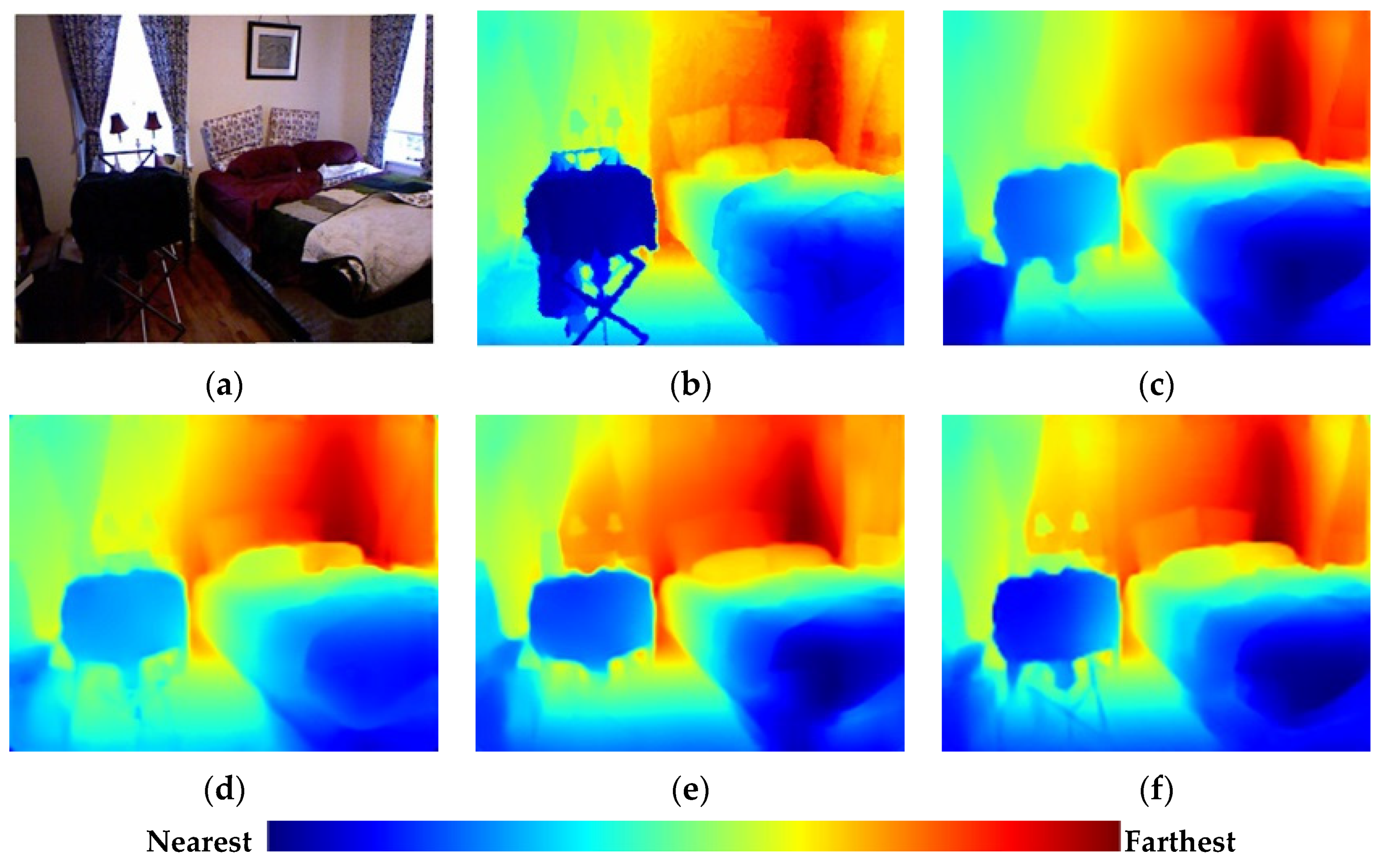
26], etc. Although great improvements have been achieved for MDE methods, reconstructing the depth for fine-grain details still requires further improvements, as shown in
Figure 1.
The current methods struggle to precisely recover large-scale geometry regions (walls) and local detail regions with rich structural information (boundaries and small parts) simultaneously, because the methods still lack the sufficient flexibility and discriminative modulation ability to handle regions with different feature information during up-sampling. This insufficiency limits the feature representation and significantly reduces the estimation accuracy in many cases.
Another area for improvement is the loss function design. Several loss function terms are commonly combined to construct loss functions for predicting a better-quality depth. Various weight-setting methods for the loss function terms have been proposed to balance the training process [
27,
28,
29], but how to enhance loss function effectiveness for fixed loss term combinations remains an open question.
Therefore, we proposed a new DCNN to settle this issue. We designed an attention-based feature distillation block (AFDB) to address the insufficiency above and integrate it into each up-sampling process in the decoder. To our best knowledge, this is the first time feature distillation has been introduced to MDE. The AFDB enriches feature representation through a series of distillation and residual asymmetric convolution (RAC) layers. We also propose a joint attention module (JAM) to adaptively and simultaneously rescale features depending on the channel and spatial contexts. The designed AFDB incorporates the proposed JAM, providing flexible and discriminative modulation to handle the features.
We also designed a wavelet-based loss function to enhance the loss function effectiveness by combining the multiple loss function with discrete wavelet transform (DWT). The estimated depth map is first divided into many patches using DWT at various frequencies, highlighting high-frequency information from depth map edge areas. The loss for each patch is then reasonably combined to generate the final loss. The experimental results verified that this loss function modification could significantly improve various metrics on benchmark datasets.
Our main contributions are summarized as follows:
A novel AFDB was designed for the proposed DCNN-based MDE method by combining feature distillation and joint attention mechanisms to boost discriminative modulation for feature processing.
A wavelet-based loss function was adopted to optimize the training by highlighting the structural detail losses and, hence, improve the estimation accuracy.
The proposed network was superior to most state-of-the-art MDE methods on two public benchmark datasets: NYU-Depth-V2 and KITTI.
4. Experiments
Section 4.1 describes the experimental setup, including the datasets, evaluation metrics, and implementation details.
Section 4.2 compares the experimental results with the current state-of-the-art methods on two public datasets: NYU-Depth-V2 [
50] (indoor scenes) and KITTI [
51] (outdoor scenes).
Section 4.3 uses the NYU-Depth-V2 dataset to analyze the effectiveness and rationality of the AFDB and wavelet-based loss function. Finally,
Section 4.4 uses cross-dataset validation on the iBims-1 [
52] dataset to assess the proposed method’s generality.
4.1. Experimental Setup
4.1.1. Datasets
The NYU-Depth-V2 dataset contains 464 indoor scenes captured by Microsoft Kinect devices. Following the official split, we used 249 scenes (approximately 50-K pair-wise images) for training and 215 scenes (654 pair-wise images) for testing.
The KITTI dataset was captured using a stereo camera and rotating LIDAR sensor mounted on a moving car. Following the commonly used Eigen split [
30], we used 22-K images from 28 scenes for training and 697 images from different scenes for testing.
iBims-1 is a high-quality RGBD dataset comprising 100 high-quality images and corresponding depth maps particularly designed to test MDE methods. A digital single-lens reflex camera and high-precision laser scanner were used to acquire the high-resolution images and highly accurate depth maps for diverse indoor scenarios. We use iBims-1 for cross-dataset validation to assess the proposed method’s generality.
4.1.2. Evaluation Metrics
The performance was quantitatively evaluated using standard metrics for these datasets, as shown below for the ground truth depth , estimated depth , and total pixels in all evaluated depth maps.
Absolute relative difference (Abs Rel):
Squared relative difference (Sq Rel):
Mean Log10 error (log10):
Root mean squared error (RMS):
Log10 root mean squared error (logRMS):
Threshold accuracy (TA):
where
The threshold accuracy is the ratio of the maximum relative error below the threshold . Conditions 1.25, 1.252, and 1.253 were used in the experiment, denoted as , , , respectively.
4.1.3. Implementation Details
The proposed model was implemented with the PyTorch [
53] framework and trained using two Nvidia RTX 2080ti graphics processing units (GPUs). The encoders were both pretrained on the ImageNet dataset [
54], and the other layers were randomly initialized. The Adam [
55] optimizer was selected with β
1 = 0.9 and β
2 = 0.999, and the weight decay = 0.0001. We set the batch size = 16 and trained the model for 20 epochs.
For the NYU-Depth-V2 dataset, we first cropped each image to 228 × 304 pixels, and the offline data augmentation methods were as the same as those of the mainstream approaches [
18,
20,
22], i.e., each training image was augmented with random scaling (0.8, 1.2), rotation (−5°, 5°), horizontal flip, rectangular window dropping, and color shift (multiplied by random value (0.8, 1.2)).
For the KITTI dataset, we masked out the sparse depth maps projected by the LIDAR point cloud and evaluated the predicted results only for valid points with ground depths. We capped the maximum estimation at the KITTI dataset maximum depth (80 m). The data augmentation methods were the same as those in [
23].
4.2. Results
Table 1 shows the evaluation metrics comparing the proposed model with several state-of-the-art methods on NYU-Depth-V2. The DenseNet-161, ResNet-101, and SENet-154 encoders were selected to verify the proposed method’s flexibility.
Figure 6 visualizes the trade-off between the performance and model parameters. The results for the comparison methods were taken from their relevant literature.
Table 1 confirms that the proposed method achieved good performances for all the encoder architectures, with the SENet-154 encoder architecture providing the best performance. The proposed method also achieved a comparable or better performance compared with the current state-of-the-art methods.
Figure 6 shows that the proposed model achieved better a trade-off between the performance and model parameters, with only the Abs Rel metric being less than [
20], but [
20] has more parameters. The proposed method with the DenseNet-161 and ResNet-101 encoders achieved better performances compared with other methods with less than 100 M parameters.
Figure 7 compares the estimated depth maps, and more qualitative results are presented in
Appendix A. The display pixels for all the estimated depth maps were the same as those for ground truth to provide easier comparisons. The proposed method achieved better geometric details and object boundaries than the other methods. Thus, the proposed method provides better fine-grain estimations.
Table 2 compares the proposed method on the KITTI test dataset using the SENet-154 encoder, with some quantitative comparisons in
Figure 8 and more qualitative results in
Appendix A. The proposed method outperforms most state-of-the-art methods and provides better object boundaries.
4.3. Algorithm Analysis
We conducted several experiments on NYU-Depth-V2 to investigate the effectiveness and rationality for the proposed AFDB and wavelet-based loss functions with the SENet-154 encoder.
4.3.1. AFDB
Figure 9 and
Table 3 compare other feature distillation methods with the proposed AFDB. Distillation steps = 4, and DWT iterations = 2 for all evaluations. All metrics are improved for the proposed AFDB at the cost of a few more model parameters. The proposed feature distillation could better predict detailed depth map characteristics.
Table 4 shows the ablation effects, i.e., distillation step and JAM influences, for the prediction results and model performance. We used two DWT iterations to decompose the depth map. More distillation steps can improve the evaluation metrics but increases the model parameters. Almost all evaluation metrics worsened for six or more distillation steps, mainly because five-step distillation generates sufficient features for subsequent treatments, and more steps just increase the local feature fusion burdens. All metrics are improved for the proposed JAM at the cost of a few more model parameters.
4.3.2. Loss Function
Table 5 shows the performance metrics for the proposed model with different loss functions for network training. We gradually added the loss terms described in
Section 3.3 to assess the loss terms selection rationality using four-step distillation as the baseline. All evaluation metrics improved with increased loss terms. Thus, the proposed loss function selection method is effective and rational.
Table 6 shows the effects from DWT iterations using the wavelet-based loss function (Equation (21)) to train the network. Three DWT iterations are sufficient to obtain the optimal results. The increased iterations reduce the performance, because the depth map size gradually reduces with the increased iterations, and the detailed depth map features from the smallest scale become indistinct, which may adversely influence the estimation quality.
4.4. Cross-Dataset Validation
We performed cross-dataset validation to assess the proposed method’s generality. We used the iBims-1 dataset, because it contains different indoor scenarios and has higher-quality depth maps closer to real depth values compared with NYU-Depth-V2. Therefore, cross-dataset validation on the iBims-1 dataset could verify the model efficiency for different data distributions between training and testing sets. The corresponding evaluation metrics are also more objective and accurate due to the higher precision depth maps.
The proposed network was first trained on NYU-Depth-V2 to generate a pretrained model. Then, the pretrained model was used without fine-tuning to estimate the iBims-1 depth maps.
Table 7 shows the corresponding evaluation metrics for iBims-1, and
Figure 10 shows some qualitative comparisons. The settings for the compared methods were the same as for the proposed method. The pretrained models for the compared methods were generated by running their open-source codes.
The test results of the pretrained models on iBims-1 were quite different from those on NYU-Depth-V2. In contrast to the earlier comparisons in
Table 1, [
17] has better performances than [
20] and [
22]. The proposed model achieved significantly better performances than the three comparative methods. Thus, the proposed method could better estimate the geometric details and object boundaries for these different scenes than the three current state-of-the-art methods.
5. Conclusions
This paper proposed a new DCNN for monocular depth estimation. Two improvements were realized compared with previous methods. We made a combination of joint attention and feature distillation mechanisms in the decoder to boost the feature discriminative modulation and proposed a wavelet-based loss function to emphasize the detailed depth map features. The experimental results on the two public datasets verified the proposed method’s effectiveness. The experiments were also conducted to verify the proposed approach effectiveness and rationality. The generality for the proposed model was demonstrated using cross-dataset validation.
Future works will focus on applying the proposed MDE methods to 3D vision applications, such as augmented reality, simultaneous localization and mapping (SLAM), and indoor scene reconstruction.


