2.3. Reflector Matching Algorithm in Initialization Mode
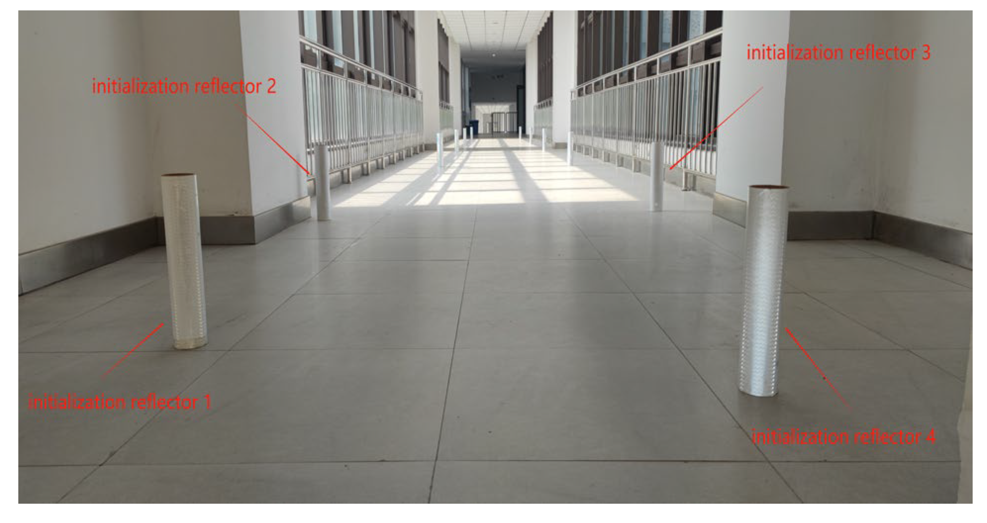
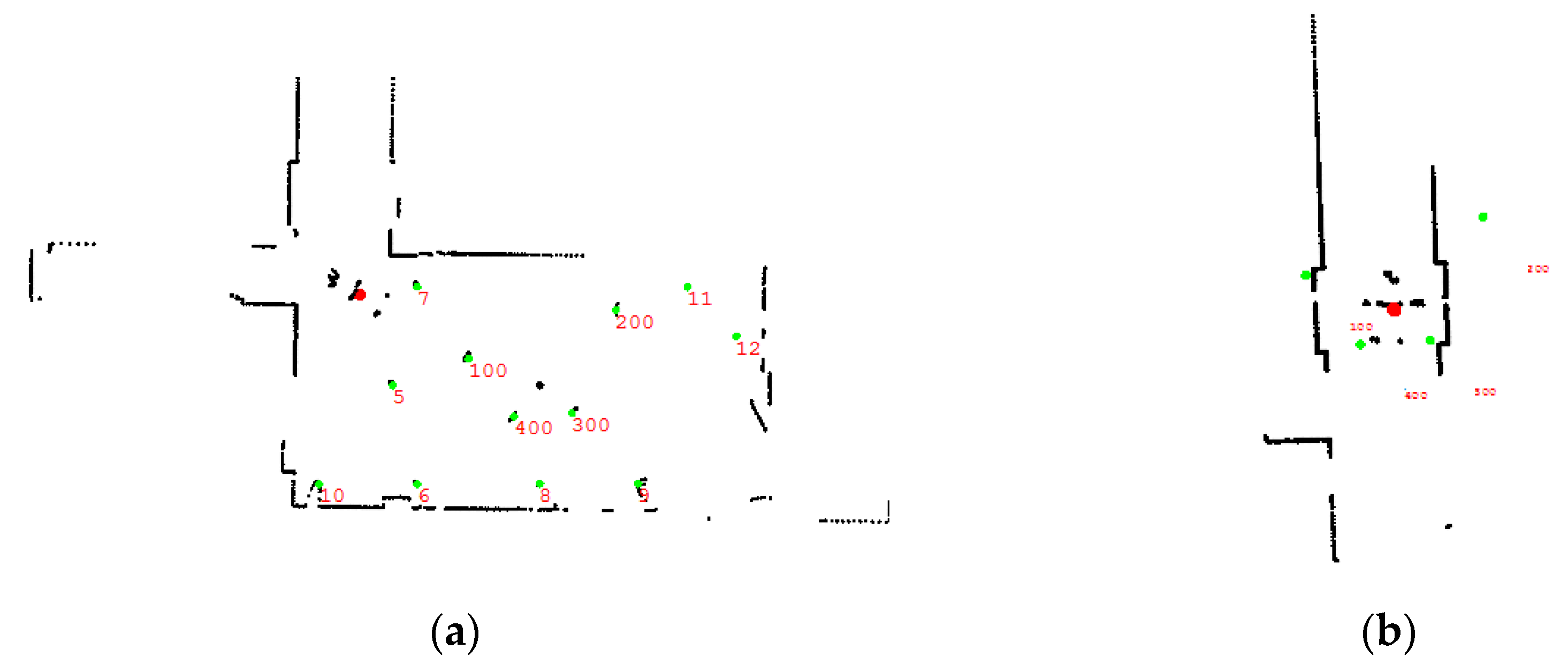
Before navigation starts, it needs to obtain the initial location and angle of the robot by running the initialization mode, and the number of initialization reflectors is at least 3 to guarantee the initial localization calculation. The initialization reflector map is a set of reflector position coordinates used to obtain the initial position calculation. The design principle of the initialization reflector should be as follows. (1) The distance difference between any two reflectors should be greater than 300 mm, and (2) the angle difference between every two reflectors should be greater than . In this step, the navigation system first finds three or more detected reflectors nearest to the mobile robot to form the candidate pool for the initial location calculation. The initial location of the mobile robot is obtained by matching the distance and angle value of the candidate pool with the referential reflector pool picked up from initialization reflector map by the simple searching mechanism.
It is assumed that there are
detected reflectors in the optimal matching area; the coordinate of the
r-th detected reflector is
, and
referential reflectors in the initialization reflector map; the coordinates of the
i-th referential reflector are
. Then, the distance vector between each two detected reflectors and each two referential reflectors can be obtained, respectively:
According to the geometric principle,
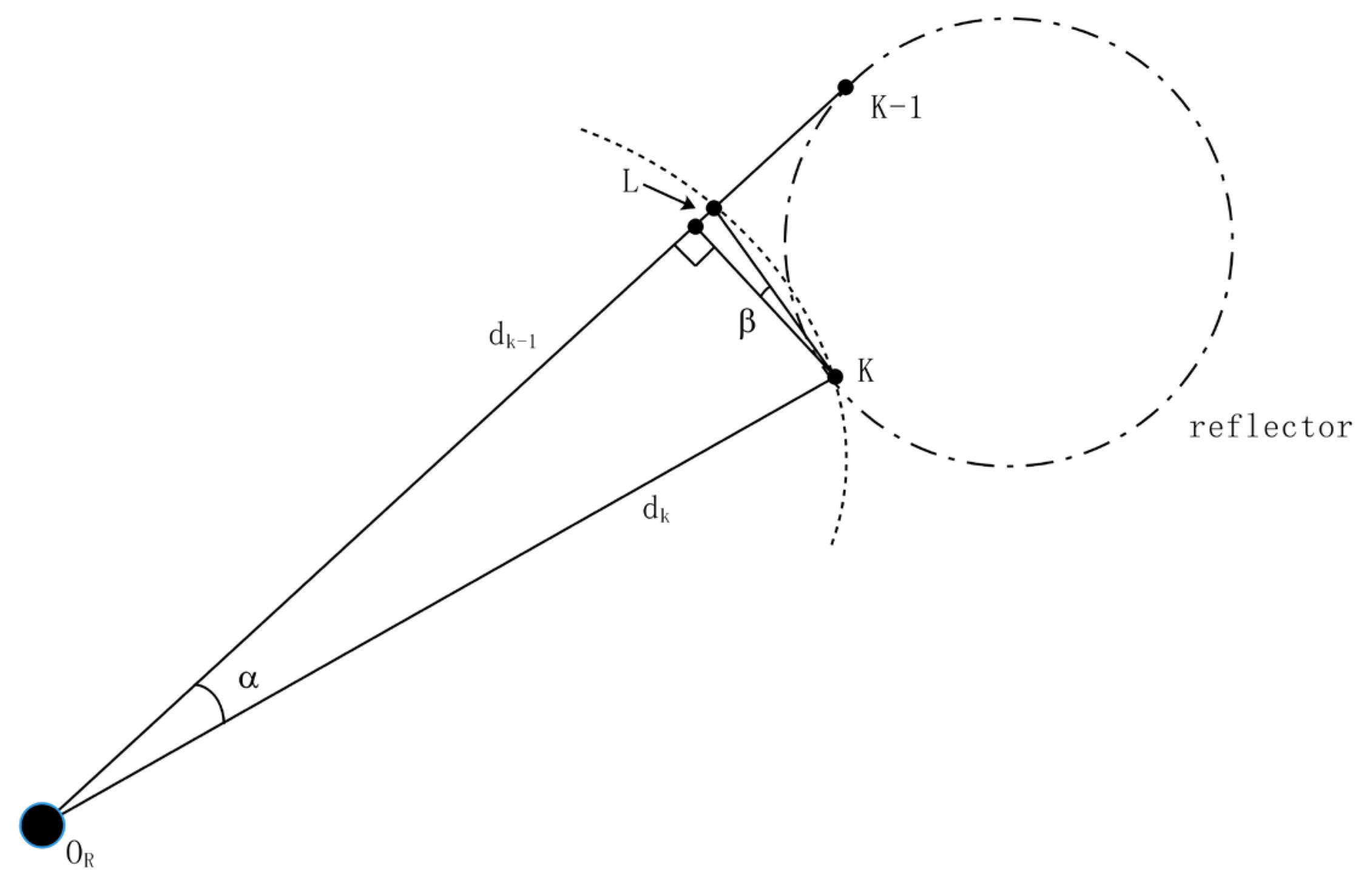
angles will be formed between any three of the N detected reflectors. Suppose that the linear distance between the
r-th detected reflector and the (
r-1)-th detected reflector is
, the one between the
r-th detected reflector and the (
r + 1)-th detected reflector is
, and the one between the (
r-1)-th detected reflector and the (
r + 1)-th detected reflector is
. The matching angle reference value
between the three detected reflectors is represented by the angle value
corresponding to the line
; we can obtain the following results:
the angle vector between each three detected reflector and each three referential reflector can be acquired, respectively:
In order to make use of the above distance vector and angle vector to match the reflector quickly and accurately, we set the distance matching error threshold as
and angle matching error threshold as
. The absolute value of the difference between each distance value of the distance vector
between the detected reflectors and each distance value of the distance vector
between the referential reflectors is calculated, and the distance difference matrix of reflector
is obtained:
where
.
Considering extreme small or large angles in the polygon are vulnerable to measurement error or noise, we only recognize the effective angle data between
. Similarly, the absolute value of the difference between each angle value of the angle vector
between the detected reflectors and each angle value of the angle vector
between the referential reflectors are calculated, and the matrix of the angle difference of the reflector
is obtained:
where
.
Take the minimum value of each column in the distance difference matrix and the angle difference matrix , compared with and respectively. If in the distance difference matrix is within , and the distance between the i-th referential reflector and the j-th detected reflector is matched successfully, then and are further compared. Therefore, the i-th referential reflector and the j-th detected reflector constitute a pair of matched reflector combinations.
2.4. Navigation Localization Algorithm
2.4.1. Motion Compensation Algorithm
Unlike the initialization mode, the navigation mode uses a guess-and-matching strategy to make the guess on the “most-possible” reflector candidates and performs the matching calculation to obtain the location. When the robot moves with low speed, the travelling distance between two adjacent points is small, so the previous location can be directly used as initial guess location for the next round of calculation. However, with the high speed or fast turning angle speed, such an assumption will introduce a distance or angle error and cannot be ignored. This section proposes a motion compensation algorithm, which effectively eliminates the odometer error caused by high-speed movement.
The navigation system first uses a motion compensation algorithm to predict the real-time pose of the mobile robot during the movement to form a desired pose sequence. The estimated location is used to complete the navigation reflector matching in the navigation mode. Since the pose history of the robot from the previous moment is known, the pose and velocity estimates of the previous moment are used to predict the pose and speed of the current moment; each time the calculation is completed, the laser odometer will be recorded to form the robot’s trajectory and rotation trajectory histogram.
Because the scanning frequency of LiDAR is high, we assume that there is no significant change in the robot’s speed and angular velocity in a scanning period, and the scanning period of LiDAR is
. In order to obtain the key parameters of the robot motion model, suppose that the pose of the robot at the last moment is
, and the time period from time zero to the previous time is divided into 2N time periods according to the scanning period; correspondingly, the velocity trajectory and rotation trajectory of the robot from time zero to the previous time are also divided into 2N sub-trajectories according to the scanning period. Here, a digital averaging filter is used to smooth out the speed changes across adjacent N calculations. Then, the horizontal velocity
, vertical velocity
, and angular velocity
at the current moment are:
where
,
are the horizontal and vertical offsets corresponding to the
i-th scan period
in the (
N~2
N)-th sub-motion trajectory;
is the angular offset corresponding to the i-th scanning period of the (
N~2
N)-th sub-rotation trajectory.
The x acceleration
, y acceleration
and angular acceleration
corresponding to the current moment are:
where
,
are the
x and
y offsets corresponding to the
i-th scan period
in the (0~
N)-th sub-motion trajectory;
is the angular offset corresponding to the
i-th scanning period of the (0~
N)-th sub-rotation trajectory.
Then, the pose of the robot at the current moment estimated by the motion compensation algorithm is
:
Due to the fact that the reflector is prone to matching failure when the robot is accelerating or decelerating, the navigation system can perform compensation calculations on the position of the detected reflectors according to the motion compensation algorithm.
Suppose that the LiDAR scans
k detected reflectors during movement, and these reflectors form a collection of detection reflectors
. Among them, the coordinate of the
j-th detected reflector in the robot coordinate system is
; then, the position
after optimizing the position of the
j-th detected reflector at the current moment by using the motion compensation algorithm is:
2.4.2. Reflector Matching Algorithm in Navigation Mode
Because the current pose can be estimated according to the motion compensation algorithm, the position of the navigation reflectors can be set arbitrarily in practical application, which can greatly reduce the complexity of setting the position of the reflector in the actual warehouse environment. The matching process of sequential comparison of distance and angle errors is cumbersome and inefficient, so the matching weight value combining distance and angle error is proposed in this part.
In the localization process, if the distance range of the detected reflectors is too large, the distance error factor in the matching weight will be dominant; if the range is too small, the angle error factor will play a leading role accordingly. Therefore, is used to screen the appropriate reflector range to balance the error factor in the matching weight. Therefore, the navigation system screens out the detected reflectors that are within the range of from the robot based on the scanning results of the LiDAR to form a set of detected reflectors and calculate the distance matrix and angle matrix between the robot and each detected reflector at this time.
In order to improve the calculation speed of the localization algorithm, it is also necessary to sort
so that the navigation system can start to match the detected reflectors close to the robot. Since the motion compensation algorithm in the previous section can estimate the current position of the robot, the navigation system can filter out the
referential reflectors in the reflector map within the range of
from the estimated position to form the referential reflectors
.The distance matrix
and the angle matrix
between the current position of the robot and each referential reflector are further calculated, and
is sorted in the same way.
The matching weight value
of the navigation reflector is calculated and compared with the weight threshold
to filter out the matching reflector combination.
Taking the minimum value of the i-th column in w, if is within the matching weight threshold , it means that the i-th reflector in the detected reflector set and the j-th reflector in the referential reflector set are successfully matched.
2.5. The Calculation of Mobile Robot’s Position
To solve the localization issue with the artificial landmark approach, most algorithms use the trilateral localization method to calculate the position of the robot in the global coordinate system [
30,
31]. However, this approach has some drawbacks. When there is a measurement error present in reflector data, the three circles do not intersect at one point anymore, and the method will fail with a large error.
The particle filter is the technique to estimate the localization from a finite set of weighted random samples to approximate the posterior probability density of any particle state [
32]. However, it heavily depends on the initial state, the number of particles used in calculation, and may have the convergence issue. For the navigation problem, except the position and angle, velocity, acceleration, and angular velocity could all be solved at the same time but require significant computing power. Quite different from particle filtering, the SVD algorithm only calculates the rotation vector and translation vector between the robot coordinate system and the global coordinate system with few computing resources. Therefore, SVD algorithm is used in this strategy to calculate the position of the robot in the global coordinate system.
During the matching process, the position matrix A of n detected reflectors and the position matrix B of n referential reflectors can be acquired; then, the rotation vector R and translation vector t of the position coordinate matrix can be calculated.
In order to calculate the rotation vector R and translation vector t, it is necessary to calculate the mean coordinates of two reflector position sets A and B; then, the mean coordinates of detected reflector position matrix A and referential reflector position matrix B are as follows:
and
are equivalent to the central coordinates of the position matrix A and B. In order to calculate the rotation vector R, it is required to eliminate the influence of the translation vector t; therefore, the above reflector position matrix should be re-centered to generate the new reflector position matrix
and
, and the covariance matrix
between the point sets should be calculated:
In the SVD algorithm,
U,
S, and
V of matrix
H can be obtained, and the optimized rotation vector
R between
A and
B can be calculated:
Ultimately, the translation vector t can be obtained by
R:
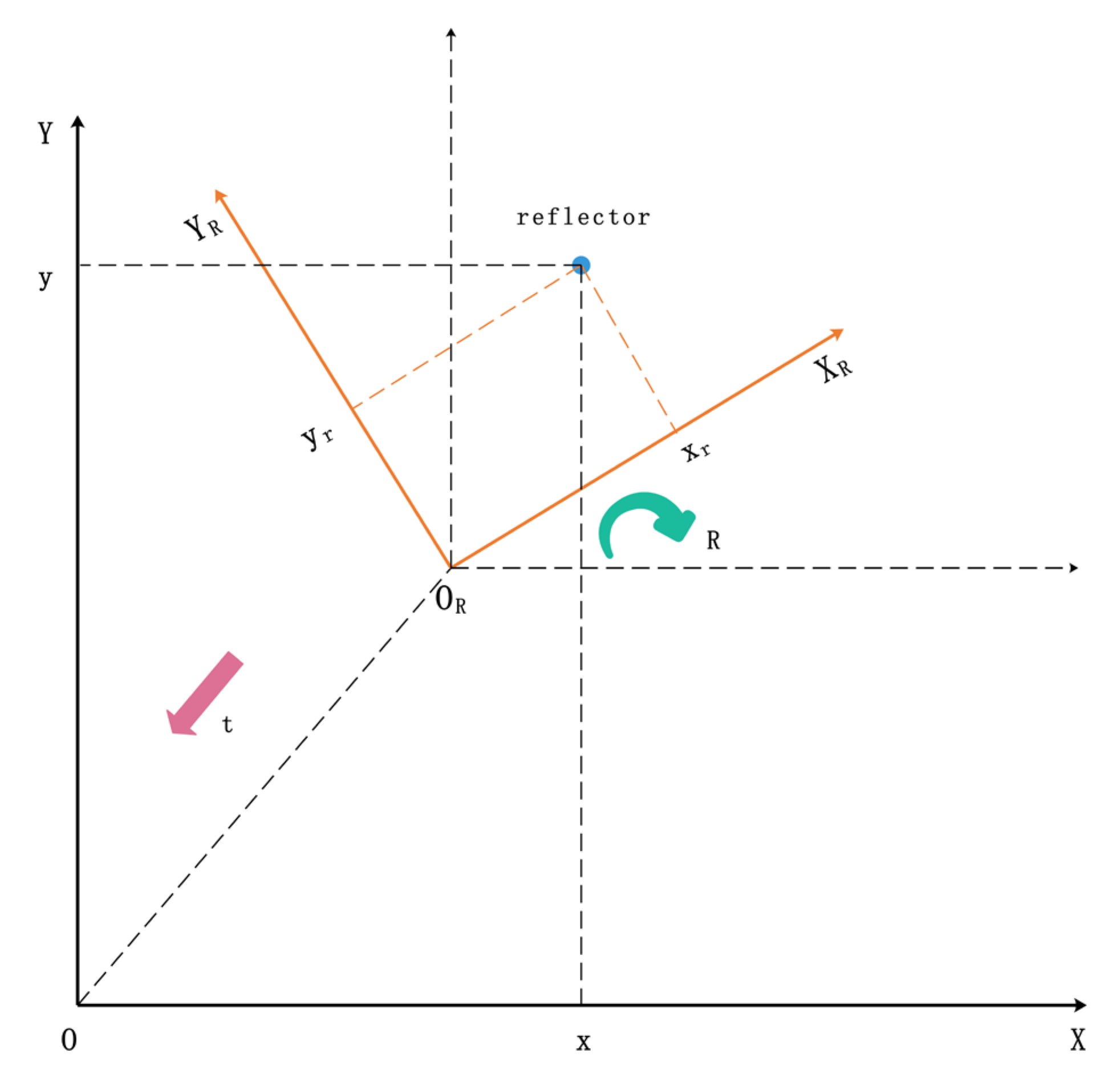
The obtained rotation vector
R and translation vector t are shown in
Figure 6. The position coordinate of the robot in the robot coordinate system is
, and the inverse operation is performed to obtain the position coordinate
in the corresponding global coordinate system:
The orientation
of the robot in the global coordinate system is as follows:


