
Cascaded Deep Learning Neural Network for Automated Liver Steatosis Diagnosis Using Ultrasound Images


Abstract
:1. Introduction
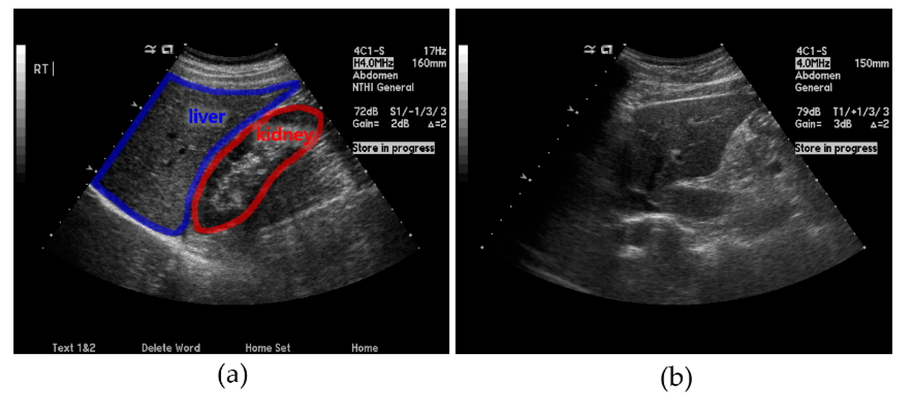
- (a)
- (b)
- Ring detection involves checking the L-K area obtained from a US image by checking for the presence of a ring that typically appears around the kidney. This method is employed for areas that are difficult to detect using only the L-K detection method described above.
- (c)
- SteatosisNet takes the above L-K areas as the input and grades the severity of fatty liver disease. It incorporates transfer learning using a CNN model called Inception v3 [30] with a dataset comprising the obtained cropped L-K areas.
2. Materials and Methods
2.1. Dataset Preparation
2.2. Preprocessing
2.3. Proposed Cascaded Deep Learning Neural Network
- (i)
- L-K detection: In this step, a pretrained deep learning neural network was used for cropping the L-K area while classifying parasagittal and non-parasagittal images.
- (ii)
- Ring detection: This step checks the parasagittal images via so-called “ring semantic segmentation (RSS),” where the presence of a ring, that is typically located around the kidney, was determined in the images.
- (iii)
- Liver steatosis grading: The SteatosisNet used an Inception V3 network [32] transfer-learned with cropped L-K images. Once being transfer-learned, the liver and kidney areas obtained from the above steps (i) and (ii) were taken as the input, and the grade of liver steatosis was determined.
2.4. Liver and Kidney (L-K) Detection
- (a)
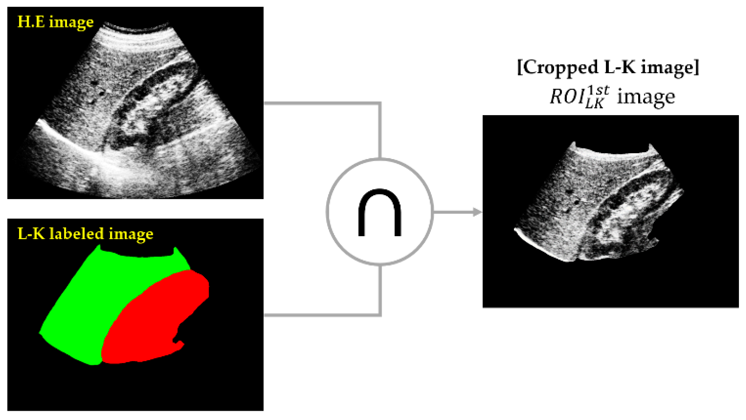
- Cropping of the L-K area: SSN was employed to obtain an L-K labeled image from a given HE image.
- (b)
- Classifying 1st parasagittal and non-parasagittal images: The output of the SSN was used as the input for the CNN, which then classified the L-K labeled image as a parasagittal or non-parasagittal image.
- (c)
- Masking operation: The logical AND operation between the L-K labeled area and HE image yielded the cropped L-K image ().
2.4.1. Cropping L-K Area
2.4.2. Classifying Parasagittal and Non-Parasagittal Images
2.4.3. Masking Operation
2.5. Ring Detection
3. Results
3.1. Performances of L-K Detection and Ring Semantic Segmentation

| Performance Deleted Extra Space | |||||
|---|---|---|---|---|---|
| Area | Mean Accuracy | Mean IOU | BF1 Score | Dataset | |
| L-K Detection | Kidney | 0.9682 | 0.8088 | 0.4650 | Training: 1590 Validation: 530 Test: 530 N:Mi:Mo:S = 30:11:10:2 |
| Liver | 0.9487 | 0.7856 | 0.5228 | ||
| Null | 0.9415 | 0.9341 | 0.8002 | ||
| Ring Detection | Kidney | 0.8642 | 0.6665 | 0.5510 | |
| Liver | 0.8318 | 0.6576 | 0.5785 | ||
| Null | 0.8318 | 0.8307 | 0.8663 | ||
| Training optimizer: Adam, Minibatch size: 8, Max epoch: 10, Learning rate of 0.001 with decay factor of 0.9, Termination condition: validation accuracy < 0.98 | |||||
3.2. Performance of SteatosisNet
3.3. Ablation Study of Our Method on SMC Database
4. Discussion and Conclusions
Author Contributions
Funding
Institutional Review Board Statement
Informed Consent Statement
Data Availability Statement
Acknowledgments
Conflicts of Interest
References
- Xiang, L.; Jia, L.S.; Shuo, H.W.; Jing, W.Z.; Qan, Q.C. Learning to Diagnose Cirrhosis with Liver Capsule Guided Ultrasound Image Classification. Sensors 2017, 17, 149. [Google Scholar]
- Kutlu, H.; Avcı, E. A Novel Method for Classifying Liver and Brain Tumors Using Convolutional Neural Networks, Discrete Wavelet Transform and Long Short-Term Memory Networks. Sensors 2019, 19, 1992. [Google Scholar] [CrossRef] [PubMed] [Green Version]
- Farrell, G.C.; Larter, C.Z. Non-alcoholic fatty liver disease: From steatosis to cirrhosis. Hepatology 2006, 43, 99–112. [Google Scholar] [CrossRef] [PubMed]
- Qian, Y.; Fan, J.G. Obesity, fatty liver and liver cancer. Hepatobiliary Pancreat. Dis. Int. 2005, 2, 173–177. [Google Scholar]
- Matthew, M.Y.; Elizabeth, M.B. Pathological aspects of fatty liver disease. Gastroenterology 2014, 147, 754–764. [Google Scholar]
- Lee, D.H. Imaging evaluation of non-alcoholic fatty liver disease: Focused on quantification. Clin. Mol. Hepatol. 2017, 4, 290–301. [Google Scholar] [CrossRef]
- Sudha, S.; Suresh, G.R.; Sukanesh, R. Speckle Noise Reduction in Ultrasound Images by Wavelet Thresholding based on Weighted Variance. Int. J. Comput. Theory Eng. 2009, 1, 7–12. [Google Scholar] [CrossRef] [Green Version]
- Jian, Y.; Jingfan, F.; Danni, A.; Xuehu, W.; Yongchang, Z.; Songyuan, T.; Yongtian, W. Local statistics and non-local mean filter for speckle noise reduction in medical ultrasound image. Neurocomputing 2016, 195, 88–95. [Google Scholar]
- FaDa, G.; Phuc, T.; ShuaiPing, G.; LiNa, Z. Anisotropic diffusion filtering for ultra-sound speckle reduction. Sci. China Technol. Sci. 2014, 57, 607–614. [Google Scholar]
- Simone, B.; Carlo, G.; Oriol, P.; Jesepa, M.; Petia, R. SRBF: Speckle reducing bilateral filtering. Ultrasound Med. Biol. 2010, 36, 1353–1363. [Google Scholar]
- Charles, A.D.; LoÏc, D.; Florence, T. Iterative weighted maximum likelihood denoising with probabilistic patch based weights. IEEE Trans. Image Process 2009, 18, 2661–2672. [Google Scholar]
- Pierrick, C.; Pierre, H.; Charles, K.; Christian, B. Nonlocal means-based speckle filtering for ultrasound images. IEEE Trans. Image Process 2009, 18, 2221–2229. [Google Scholar]
- Sara, P.; Mariana, P.; Cesario, V.A.; Luisa, V. A nonlocal SAR image de-noising algorithm based on LLMMSE wavelet shrinkage. IEEE Trans. Geosci. Remote Sens. 2012, 50, 606–616. [Google Scholar]
- Nedumaran, D.; Sivakumar, R.; Sekar, V.; Gayathri, K.M. Speckle noise reduction in ultrasound biomedical B-scan images using discrete topological derivative. Ultrasound Med. Biol. 2012, 38, 276–286. [Google Scholar]
- Shan, G.; Boyu, Z.; Cihui, Y.; Lei, Y. Speckle noise reduction in medical ultrasound image using monogenic wavelet and Laplace mixture distribution. Digit. Signal Process. 2018, 72, 192–207. [Google Scholar]
- Richard, H.M.; Marna, E.; Edward, I.B.; Paul, M.G. Hepatorenal Index as an Accurate, Simple, and Effective Tool in Screening for Steatosis. Am. J. Roentgenol. 2012, 199, 997–1002. [Google Scholar]
- Webb, M.; Yeshua, H.; Zelber-Sagi, S.; Santo, E.; Brazowski, E.; Halpern, Z.; Oren, R. Diagnostic value of a computerized hepatorenal index for sonographic quantification of liver steatosis. Am. J. Roentgenol. 2009, 192, 909–914. [Google Scholar] [CrossRef] [Green Version]
- Robert, M.H.; Shanmugam, K.; Dinstein, I.H. Textural features for image classification. IEEE Trans. Syst. Man Cybern. 1973, 6, 610–621. [Google Scholar]
- Andrade, A.; Silva, J.S.; Santos, J.; Belo-Soares, P. Classifier approaches for liver steatosis using ultrasound images. Procedia Technol. 2012, 5, 763–770. [Google Scholar] [CrossRef] [Green Version]
- Rivas, E.C.; Moreno, F.; Benitez, A.; Morocho, V.; Vanegas, P.; Medina, R. Hepatic Steatosis detection using the co-occurrence matrix in tomography and ultrasound images. Signal. Process Images Comput. Vis. 2015, 1–7. [Google Scholar] [CrossRef] [Green Version]
- Lei, Z.; Haijiang, Z.; Tengfei, Y. Deep Neural Networks for fatty liver ultrasound images classification. Chin. Control. Decis. Conf. 2019, 4641–4646. [Google Scholar] [CrossRef]
- Michał, B.; Grzegorz, S.; Cezary, S.; Piotr, K.; Łukasz, M.; Rafał, P.; Bogna, Z.W.; Krzysztof, Z.; Piotr, S.; Andrzej, N. Transfer learning with deep convolutional neural network for liver steatosis assessment in ultrasound images. Int. J. Comput. Assist. Radiol. Surg. 2018, 13, 1895–1903. [Google Scholar]
- Fuzhen, Z.; Zhiyuan, Q.; Keyu, D.; Dongbo, X.; Yongchun, Z.; Hengshu, Z.; Hui, X.; Qing, H. A Comprehensive Survey on Transfer Learning. arXiv 2020, arXiv:1911.02685. [Google Scholar]
- Chuanqi, T.; Fuchun, S.; Tao, K.; Wenchang, Z.; Chao, Y.; Chunfang, L. A Survey on Deep Transfer Learning. arXiv 2018, arXiv:1808.01974. [Google Scholar]
- Wen, C.; Xing, A.; Longfei, C.; Chaoyang, L.; Qian, Z.; Ruijun, G. Application of Deep Learning in Quantitative Analysis of 2-Dimensional Ultrasound Imaging of Nonalcoholic Fatty Liver Disease. J. Ultrasound Med. 2019, 39, 51–59. [Google Scholar]
- Elena, C.C.; Anca-Loredana, U.; Ștefan, C.U.; Andreea, V.I.; Lucian, G.G.; Gabriel, G.; Larisa, S.; Adrian, S. Transfer learning with pre-trained deep convolutional neural networks for the automatic assessment of liver steatosis in ultrasound images. Med. Ultrason. 2020, 23, 135–139. [Google Scholar]
- Zamanian, H.; Mostaar, A.; Azadeh, P.; Ahmadi, M. Implementation of Combinational Deep Learning Algorithm for Non-alcoholic Fatty Liver Classification in Ultrasound Images. J. Biomed. Phys. Eng. 2021, 11, 73–84. [Google Scholar] [CrossRef] [PubMed]
- Liang-Chieh, C.; Yukun, Z.; George, P.; Florian, S.; Hartwig, A. Encoder-Decoder with Atrous Separable Convolution for Semantic Image Segmentation. arXiv 2018, arXiv:1802.02611. [Google Scholar]
- Imad, M.; Doukhi, O.; Lee, D.-J. Transfer Learning Based Semantic Segmentation for 3D Object Detection from Point Cloud. Sensors 2021, 21, 3964. [Google Scholar] [CrossRef] [PubMed]
- Christian, S.; Vincent, V.; Sergey, I.; Jon, S.; Zbigniew, W. Rethinking the Inception Architecture for Computer Vision. arXiv 2015, arXiv:1512.00567. [Google Scholar]
- Nema, S.; Hebatullah, M.; Asmaa, S. Medical image enhancement based on histogram algorithms. Procedia Comput. Sci. 2019, 163, 300–311. [Google Scholar]
- Nasser, A.; Amr, A.; AbdAllah, A.E.; Ahmed, A. Efficient 3D Deep Learning Model for Medical Image Semantic Segmentation. Alex. Eng. J. 2021, 60, 1231–1239. [Google Scholar]
- Ravi, S.; Am, K. Morphological Operations for Image Processing: Understanding and its Applications. Natl. Conf. VLSI Signal. Process. Commun. 2013, 13, 17–19. [Google Scholar]
- Vargas Rivero, J.R.; Gerbich, T.; Buschardt, B.; Chen, J. Data Augmentation of Automotive LIDAR Point Clouds under Adverse Weather Situations. Sensors 2021, 21, 4503. [Google Scholar] [CrossRef] [PubMed]


| Data Source | Training (60%) | Validation (20%) | Test (20%) | US Machine | |||||||||
|---|---|---|---|---|---|---|---|---|---|---|---|---|---|
| N | Mi | Mo | S | N | Mi | Mo | S | N | Mi | Mo | S | ||
| Sasung | 900 | 330 | 300 | 60 | 300 | 110 | 100 | 20 | 300 | 110 | 100 | 20 | ACUSON Sequoia 512 |
| Byra [22] | 102 | 114 | 54 | 60 | 34 | 38 | 18 | 20 | 34 | 38 | 18 | 20 | GE Vivid E9 |
| Total | 1902 | 444 | 594 | 180 | 634 | 148 | 198 | 60 | 634 | 148 | 198 | 60 | -- |
| Reference | Model | Accuracy | Sensitivity | Specificity | |
|---|---|---|---|---|---|
| Andrea et al. [20] | KNN (1) | 74.05% | - | - | |
| Zhang et al. [21] | CNN (2) | 90.00% | 81.00% | 92.00% | |
| Byra et al. [22] | CNN (3) | 96.30% | 100.00% | 88.20% | |
| Cao et al. [23] | CNN (4) | 73.97% | - | - | |
| Anca et al. [24] | CNN (5) | 93.23% | 88.90% | - | |
| Zamanian et al. [25] | CNN (6) | 98.64% | 97.20% | 100.00% | |
| Proposed methods | Cascaded NN | ♠ | 99.91% | 99.78% | 100.00% |
| ♥ | 100.00% | 100.00% | 100.00% | ||
| ♣ | 99.62% | 99.13% | 100.00% | ||
| ♦ | 100.00% | 100.00% | 100.00% | ||
| Ablated Components | Accuracy | Sensitivity | Specificity |
|---|---|---|---|
| Only Ring | 98.50% | 98.50% | 97.17% |
| Only L-K | 96.89% | 97.83% | 95.65% |
| Ring + L-K | 95.38% | 95.77% | 95.09% |
| Nothing | 99.91% | 99.78% | 100.00% |
Publisher’s Note: MDPI stays neutral with regard to jurisdictional claims in published maps and institutional affiliations. |
© 2021 by the authors. Licensee MDPI, Basel, Switzerland. This article is an open access article distributed under the terms and conditions of the Creative Commons Attribution (CC BY) license (https://creativecommons.org/licenses/by/4.0/).
Share and Cite
Rhyou, S.-Y.; Yoo, J.-C. Cascaded Deep Learning Neural Network for Automated Liver Steatosis Diagnosis Using Ultrasound Images. Sensors 2021, 21, 5304. https://doi.org/10.3390/s21165304
Rhyou S-Y, Yoo J-C. Cascaded Deep Learning Neural Network for Automated Liver Steatosis Diagnosis Using Ultrasound Images. Sensors. 2021; 21(16):5304. https://doi.org/10.3390/s21165304
Chicago/Turabian StyleRhyou, Se-Yeol, and Jae-Chern Yoo. 2021. "Cascaded Deep Learning Neural Network for Automated Liver Steatosis Diagnosis Using Ultrasound Images" Sensors 21, no. 16: 5304. https://doi.org/10.3390/s21165304
APA StyleRhyou, S.-Y., & Yoo, J.-C. (2021). Cascaded Deep Learning Neural Network for Automated Liver Steatosis Diagnosis Using Ultrasound Images. Sensors, 21(16), 5304. https://doi.org/10.3390/s21165304