An Automated Light Trap to Monitor Moths (Lepidoptera) Using Computer Vision-Based Tracking and Deep Learning

 ,
,  ,
, 
Abstract
:1. Introduction
2. Materials and Methods
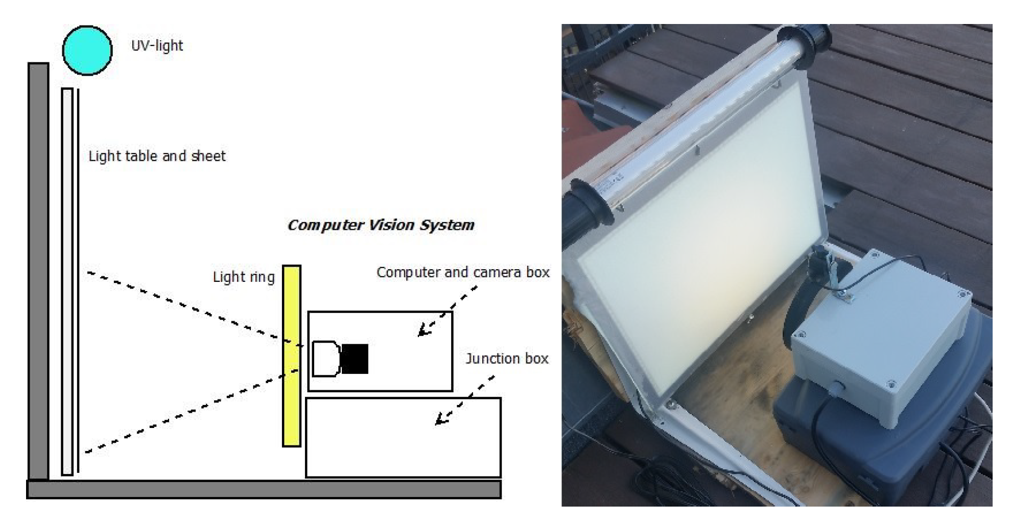
2.1. Hardware Solution
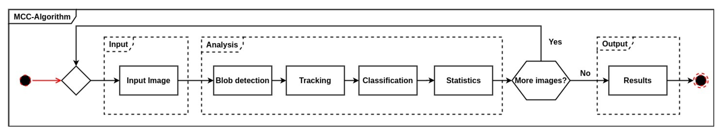
2.2. Counting and Classification of Moths
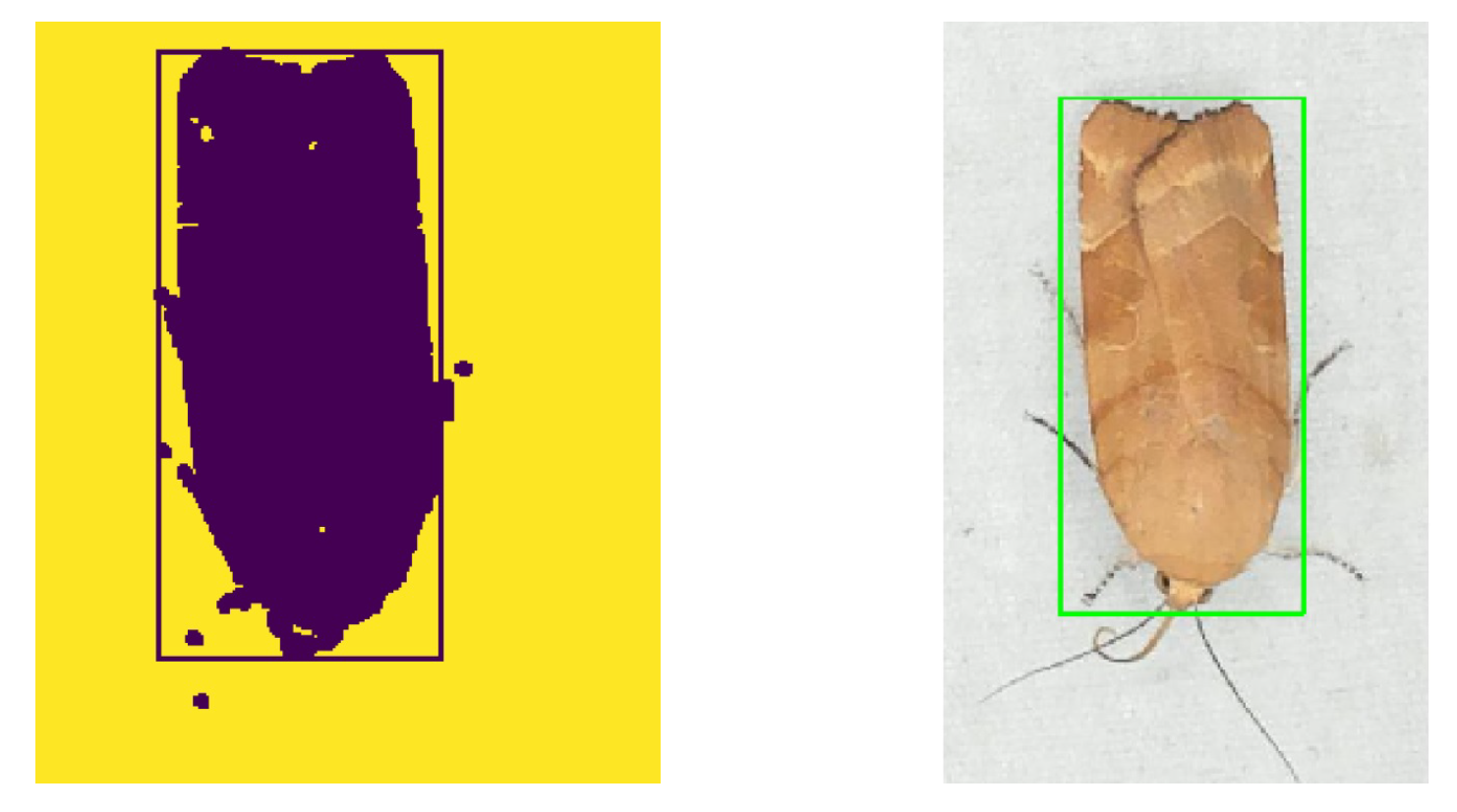
2.2.1. Blob Detection and Segmentation
2.2.2. Insect Tracking and Counting
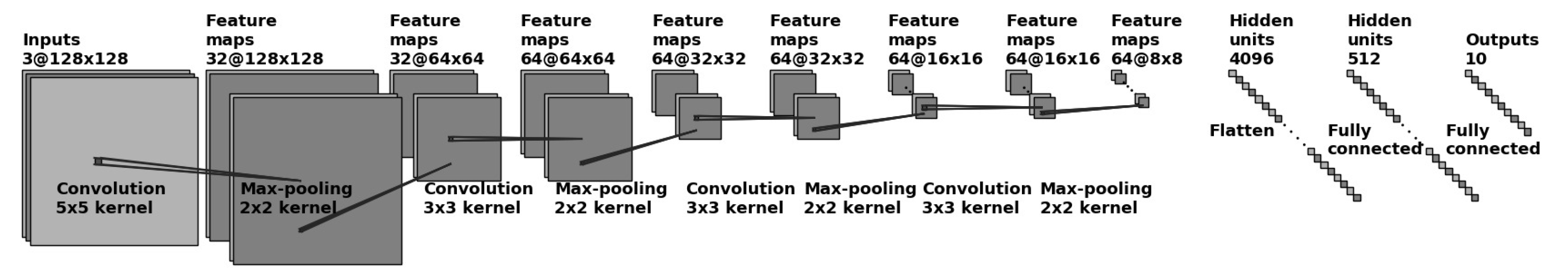
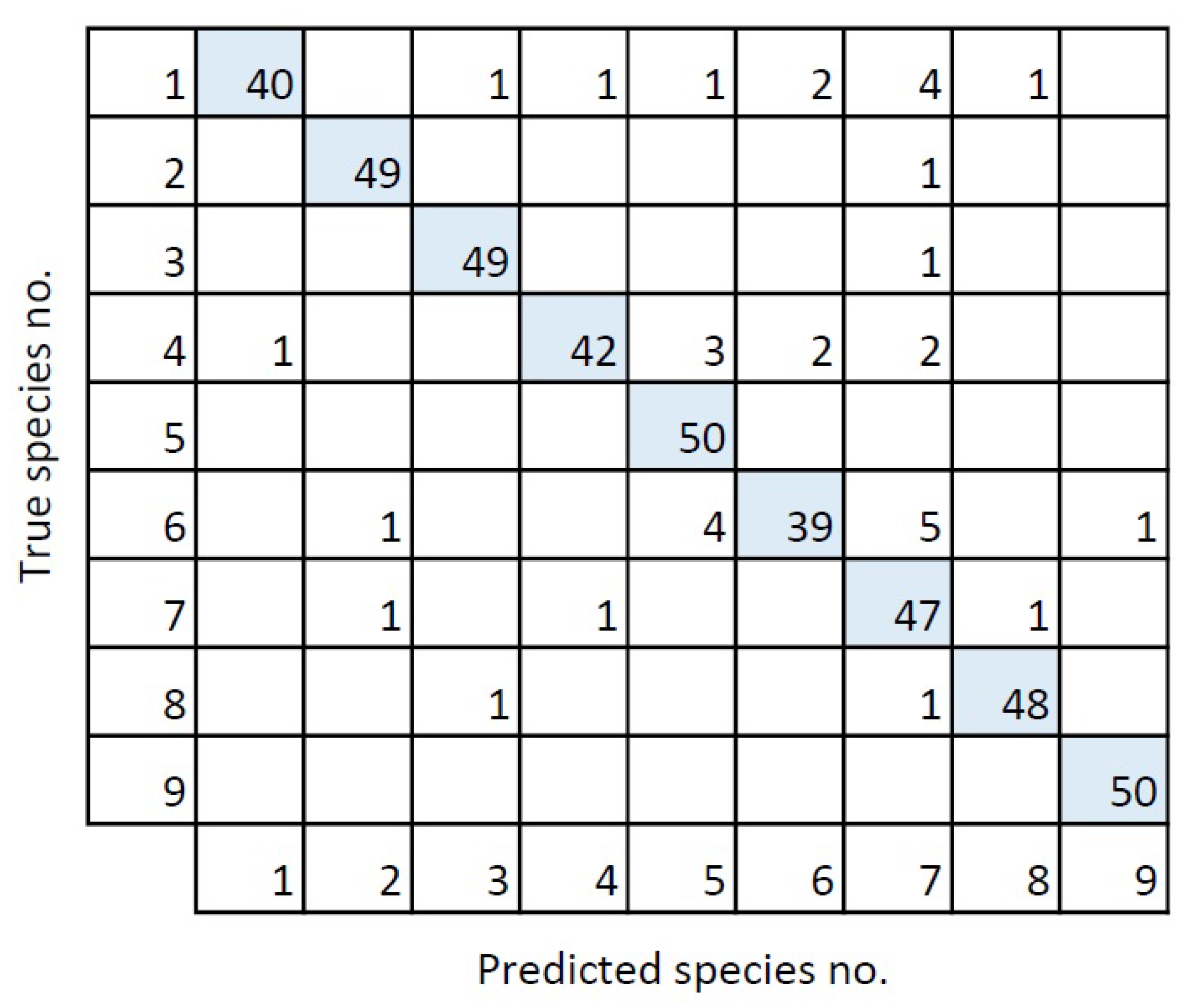
2.2.3. Moth Species Classification
- Fixed pool size and stride, ,
- Kernel size ,
- Convolutional depth n,
- Fully connected size n,
- Optimizer n,
2.2.4. Summary Statistics
2.3. Experiment
3. Results
3.1. Insect Tracking and Counting
3.2. Summary Statistics
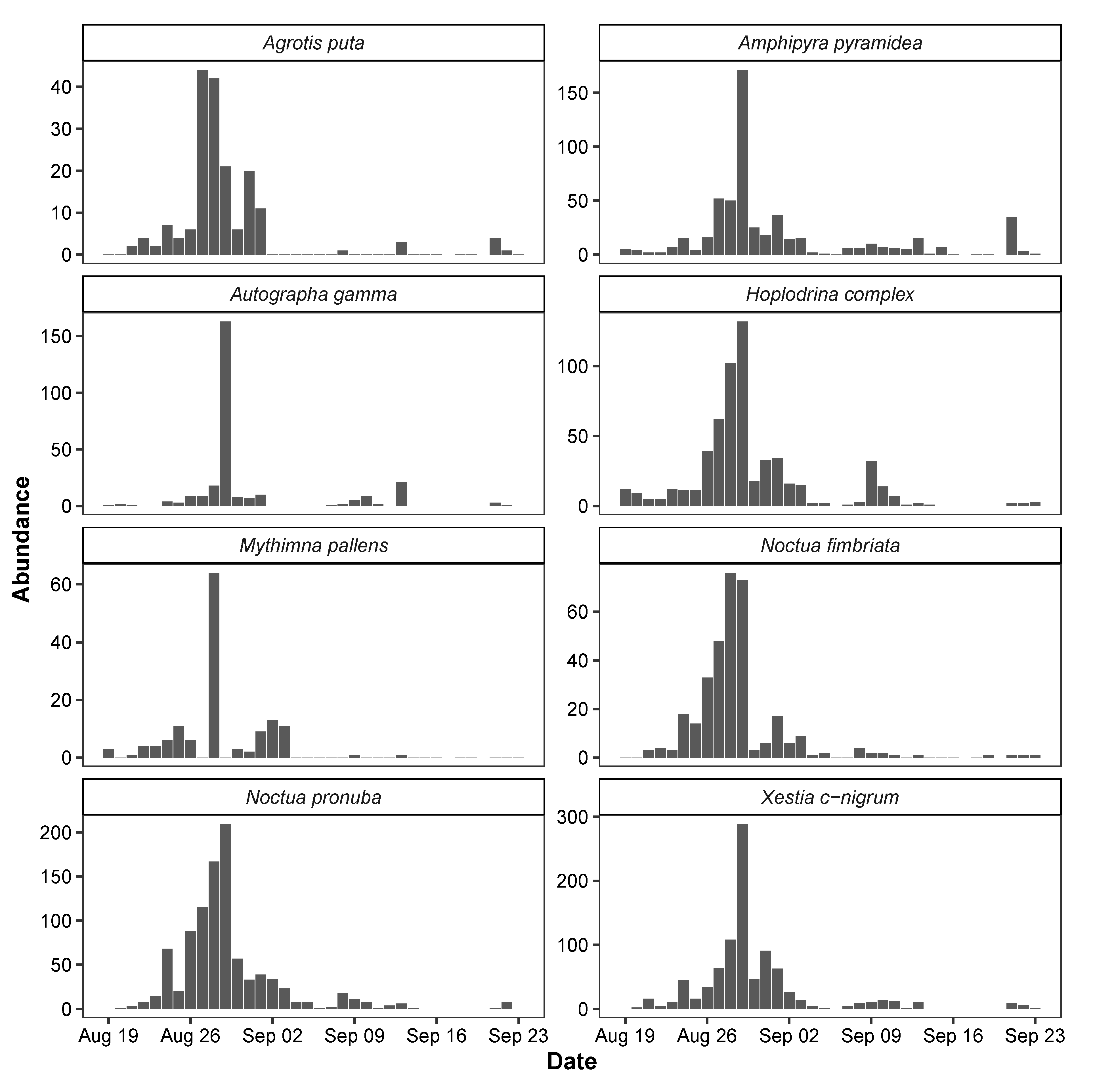
3.3. Temporal Variation in Moth Abundance
4. Discussion
5. Conclusions
Author Contributions
Funding
Data Availability Statement
Acknowledgments
Conflicts of Interest
References
- Hallmann, C.A.; Sorg, M.; Jongejans, E.; Siepel, H.; Hofland, N.; Schwan, H.; Stenmans, W.; Müller, A.; Sumser, H.; Hörren, T.; et al. More than 75 percent decline over 27 years in total flying insect biomass in protected areas. PLoS ONE 2017, 12, e0185809. [Google Scholar] [CrossRef] [PubMed] [Green Version]
- Harvey, J.; Heinen, R.; Armbrecht, I.E.A. International scientists formulate a roadmap for insect conservation and recovery. Nat. Ecol. Evol. 2020, 4, 174–176. [Google Scholar] [CrossRef] [PubMed]
- Fox, R.; Parsons, M.; Chapman, J. The State of Britain’s Larger Moths 2013; Technical Report; 2013; Available online: https://butterfly-conservation.org/moths/the-state-of-britains-moths (accessed on 9 November 2020).
- Franzén, M.; Johannesson, M. Predicting extinction risk of butterflies and moths (Macrolepidoptera) from distribution patterns and species characteristics. J. Insect Conserv. 2007, 11, 367–390. [Google Scholar] [CrossRef]
- Groenendijk, D.; Ellis, W.N. The state of the Dutch larger moth fauna. J. Insect Conserv. 2011, 15, 95–101. [Google Scholar] [CrossRef]
- Macgregor, C.J.; Williams, J.H.; Bell, J.R.; Thomas, C.D. Moth biomass increases and decreases over 50 years in Britain. Nat. Ecol. Evol. 2019, 3, 1645–1649. [Google Scholar] [CrossRef]
- Klapwijk, M.J.; Csóka, G.; Hirka, A.; Bjöorkman, C. Forest insects and climate change: Long-term trends in herbivore damage. Ecol. Evol. 2013, 3, 4183–4196. [Google Scholar] [CrossRef] [Green Version]
- Furlong, M.J.; Wright, D.J.; Dosdall, L.M. Diamondback moth ecology and management: Problems, progress, and prospects. Annu. Rev. Entomol. 2013, 58, 517–541. [Google Scholar] [CrossRef]
- Jonason, D.; Franzén, M.; Ranius, T. Surveying moths using light traps: Effects of weather and time of year. PLoS ONE 2014, 9, e92453. [Google Scholar] [CrossRef]
- Ding, W.; Taylor, G. Automatic moth detection from trap images for pest management. Comput. Electron. Agric. 2016, 123, 17–28. [Google Scholar] [CrossRef] [Green Version]
- Watson, A.; O’neill, M.; Kitching, I. Automated identification of live moths (Macrolepidoptera) using digital automated identification system (DAISY). Syst. Biodivers. 2004, 1, 287–300. [Google Scholar] [CrossRef]
- Mayo, M.; Watson, A.T. Automatic species identification of live moths. Knowl. Based Syst. 2007, 20, 195–202. [Google Scholar] [CrossRef] [Green Version]
- Batista, G.E.; Campana, B.; Keogh, E. Classification of live moths combining texture, color and shape primitives. In Proceedings of the 9th International Conference on Machine Learning and Applications, ICMLA 2010, Washington, DC, USA, 12–14 December 2010. [Google Scholar] [CrossRef]
- Chang, Q.; Qu, H.; Wu, P.; Yi, J. Fine-Grained Butterfly and Moth Classification Using Deep Convolutional Neural Networks; Rutgers University: New Brunswick, NJ, USA, 2017. [Google Scholar]
- Simonyan, K.; Zisserman, A. Very deep convolutional networks for large-scale image recognition. In Proceedings of the 3rd International Conference on Learning Representations, ICLR 2015—Conference Track Proceedings, San Diego, CA, USA, 7–9 May 2015. [Google Scholar]
- Szegedy, C.; Liu, W.; Jia, Y.; Sermanet, P.; Reed, S.; Anguelov, D.; Erhan, D.; Vanhoucke, V.; Rabinovich, A. Going deeper with convolutions. In Proceedings of the IEEE Computer Society Conference on Computer Vision and Pattern Recognition 2015, Boston, MA, USA, 7–12 June 2015. [Google Scholar]
- He, K.; Zhang, X.; Ren, S.; Sun, J. Deep residual learning for image recognition. In Proceedings of the IEEE Computer Society Conference on Computer Vision and Pattern Recognition 2016, Las Vegas, NV, USA, 27–30 June 2016. [Google Scholar]
- Xia, D.; Chen, P.; Wang, B.; Zhang, J.; Xie, C. Insect detection and classification based on an improved convolutional neural network. Sensors 2018, 18, 4169. [Google Scholar] [CrossRef] [PubMed] [Green Version]
- Zhong, Y.; Gao, J.; Lei, Q.; Zhou, Y. A vision-based counting and recognition system for flying insects in intelligent agriculture. Sensors 2018, 18, 1489. [Google Scholar] [CrossRef] [PubMed] [Green Version]
- Redmon, J.; Divvala, S.; Girshick, R.; Farhadi, A. You only look once: Unified, real-time object detection. In Proceedings of the IEEE Computer Society Conference on Computer Vision and Pattern Recognition 2016, Las Vegas, NV, USA, 27–30 June 2016. [Google Scholar]
- Roosjen, P.P.; Kellenberger, B.; Kooistra, L.; Green, D.R.; Fahrentrapp, J. Deep learning for automated detection of Drosophila suzukii: Potential for UAV-based monitoring. Pest Manag. Sci. 2020. [Google Scholar] [CrossRef]
- Eliopoulos, P.; Tatlas, N.A.; Rigakis, I.; Potamitis, I. A “smart” trap device for detection of crawling insects and other arthropods in urban environments. Electron. (Switz.) 2018, 7, 161. [Google Scholar] [CrossRef] [Green Version]
- Bioform. Leucht-Kleinanlage 12V, 15W Superaktinisch. Available online: https://www.bioform.de/ (accessed on 9 November 2020).
- Computermester. A3 LED Light Table. Available online: https://www.computermester.dk/shop/lysborde-214c1.html (accessed on 9 November 2020).
- 24hshop. USB LED Light Ring. Available online: https://www.24hshop.dk/mobiltilbehor/iphone-tilbehor/iphone-ovrigt/usb-led-ring-belysning (accessed on 9 November 2020).
- Logitech. Brio Ultra HD Pro Webcam. Available online: https://www.logitech.com/en-us/product/brio (accessed on 9 November 2020).
- Motion. Open Source Program that Monitors Video Signals from Many Types of Cameras. Available online: https://motion-project.github.io/ (accessed on 20 December 2020).
- Otsu, N. Threshold selection method from gray-level histograms. IEEE Trans Syst Man Cybern 1979, 9, 62–66. [Google Scholar] [CrossRef] [Green Version]
- Munkres, J. Algorithms for the Assignment and Transportation Problems. J. Soc. Ind. Appl. Math. 1957, 5, 32–38. [Google Scholar] [CrossRef] [Green Version]
- Bashir, F.; Porikli, F. Performance Evaluation of Object Detection and Tracking Systems. Mitsubishi Electr. Res. Lab. 2006, TR2006-041. Available online: https://www.researchgate.net/publication/237749648_Performance_Evaluation_of_Object_Detection_and_Tracking_Systems (accessed on 9 November 2020).
- Liu, W.; Wang, Z.; Liu, X.; Zeng, N.; Liu, Y.; Alsaadi, F.E. A survey of deep neural network architectures and their applications. Neurocomputing 2017, 234, 11–26. [Google Scholar] [CrossRef]
- Bjerge, K.; Frigaard, C.E.; Mikkelsen, P.H.; Nielsen, T.H.; Misbih, M.; Kryger, P. A computer vision system to monitor the infestation level of Varroa destructor in a honeybee colony. Comput. Electron. Agric. 2019, 164, 104898. [Google Scholar] [CrossRef]
- Sandler, M.; Howard, A.; Zhu, M.; Zhmoginov, A.; Chen, L.C. MobileNetV2: Inverted Residuals and Linear Bottlenecks. In Proceedings of the IEEE Computer Society Conference on Computer Vision and Pattern Recognition 2018, Salt Lake City, UT, USA, 18–22 June 2018. [Google Scholar]
- Krizhevsky, A.; Sutskever, I.; Hinton, G.E. ImageNet classification with deep convolutional neural networks. Commun. ACM 2017, 60, 84–90. [Google Scholar] [CrossRef]
- Huang, Y.Y.; Wang, W.Y. Deep residual learning for weakly-supervised relation extraction. In Proceedings of the EMNLP 2017—Conference on Empirical Methods in Natural Language Processing, Copenhagen, Denmark, 7–11 September 2017. [Google Scholar]
- Tan, M.; Le, Q.V. EfficientNet: Rethinking Model Scaling for Convolutional Neural Networks. arXiv 2019, arXiv:1905.11946. [Google Scholar]
- Huang, G.; Liu, Z.; Weinberger, K.Q. Densely Connected Convolutional Networks. arXiv 2016, arXiv:1608.06993. [Google Scholar]
- Wu, S.; Zhong, S.; Liu, Y. ResNet. Multimed. Tools Appl. 2017. [Google Scholar] [CrossRef]
- Szegedy, C.; Vanhoucke, V.; Ioffe, S.; Shlens, J.; Wojna, Z. Rethinking the Inception Architecture for Computer Vision. In Proceedings of the 2016 IEEE Conference on Computer Vision and Pattern Recognition (CVPR), Las Vegas, NV, USA, 26 June–1 July 2016; pp. 2818–2826. [Google Scholar]
- R Core Team. R: A Language and Environment for Statistical Computing; R Core Team: Geneva, Switzerland, 2020; Available online: http://softlibre.unizar.es/manuales/aplicaciones/r/fullrefman.pdf (accessed on 9 November 2020).
- Thomsen, P.F.; Jørgensen, P.S.; Bruun, H.H.; Pedersen, J.; Riis-Nielsen, T.; Jonko, K.; Słowińska, I.; Rahbek, C.; Karsholt, O. Resource specialists lead local insect community turnover associated with temperature—Analysis of an 18-year full-seasonal record of moths and beetles. J. Anim. Ecol. 2016, 85, 251–261. [Google Scholar] [CrossRef]
- Høye, T.T.; Ärje, J.; Bjerge, K.; Hansen, O.L.P.; Iosifidis, A.; Leese, F.; Mann, H.M.R.; Meissner, K.; Melvad, C.; Raitoharju, J. Deep learning and computer vision will transform entomology. PNAS 2020, in press. [Google Scholar] [CrossRef]


| No. | Species | Numbers |
|---|---|---|
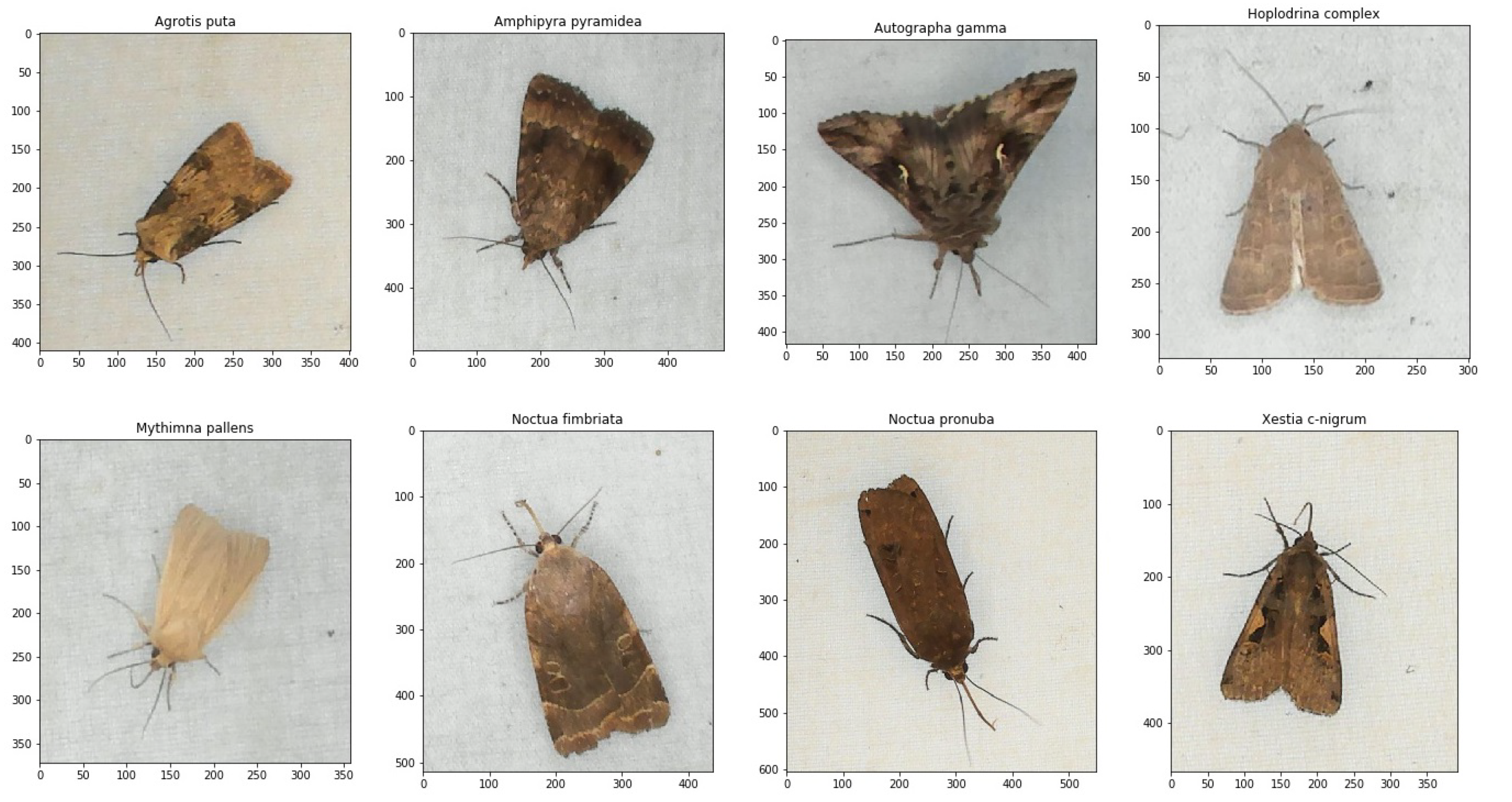
| 1 | Agrotis puta | 250 |
| 2 | Amphipyra pyramidea | 250 |
| 3 | Autographa gamma | 250 |
| 4 | Hoplodrina complex | 250 |
| 5 | Mythimna pallens | 250 |
| 6 | Noctua fimbriata | 250 |
| 7 | Noctua pronuba | 250 |
| 8 | Xestia c-nigrum | 250 |
| 9 | Vespula vulgaris | 250 |
| Total | 2250 |
| Rating | Hyperparameters | Learnable Parameters | -Score |
|---|---|---|---|
| 1. | 3, 3, 32, 128, 512 | 4,330,122 | 0.942 |
| 2. | 5, 1, 32, 128, 512 | 4,266,122 | 0.929 |
| 3. | 5, 3, 32, 64, 512 | 2,197,578 | 0.928 |
| 4. | 3, 3, 32, 64, 512 | 2,196,042 | 0.923 |
| 5. | 5, 3, 32, 128, 512 | 4,331,658 | 0.922 |
| ... | |||
| 31. | 5, 1, 64, 64, 512 | 2,185,674 | 0.871 |
| 32. | 5, 3, 32, 32, 512 | 2,164,810 | 0.871 |
| 33. | 5, 3, 64, 128, 512 | 4,352,522 | 0.853 |
| 34. | 5, 3, 32, 128, 512 | 4,331,658 | 0.853 |
| ... | |||
| 62. | 5, 1, 64, 64, 512 | 2,185,674 | 0.749 |
| 63. | 3, 3, 64, 64, 256 | 1,163,978 | 0.737 |
| 64. | 3, 3, 64, 64, 512 | 2,215,370 | 0.682 |
| Metric | Equation | Result |
|---|---|---|
| TDR | (6) | 0.79 |
| FAR | (5) | 0.22 |
| Moth Species | GT | TP | FP | FN |
|---|---|---|---|---|
| Agrotis puta | 32 | 24 | 6 | 8 |
| Amphipyra pyramidea | 13 | 11 | 50 | 2 |
| Autographa gamma | 6 | 5 | 9 | 1 |
| Hoplodrina complex | 77 | 63 | 14 | 14 |
| Mythimna pallens | 5 | 5 | 10 | 0 |
| Noctua fimbriata | 18 | 16 | 9 | 2 |
| Noctua pronuba | 93 | 68 | 32 | 25 |
| Xestia c-nigrum | 184 | 156 | 18 | 28 |
| Unknown | 57 | 9 | 10 | 48 |
| Total | 485 | 357 | 168 | 128 |
| Moth Species | Precision | Recall | -score |
|---|---|---|---|
| Agrotis puta | 0.80 | 0.75 | 0.77 |
| Amphipyra pyramidea | 0.18 | 0.85 | 0.30 |
| Autographa gamma | 0.36 | 0.83 | 0.50 |
| Hoplodrina complex | 0.82 | 0.82 | 0.82 |
| Mythimna pallens | 0.33 | 1.00 | 0.50 |
| Noctua fimbriata | 0.65 | 0.89 | 0.74 |
| Noctua pronuba | 0.68 | 0.73 | 0.70 |
| Xestia c-nigrum | 0.90 | 0.85 | 0.87 |
| Unknown | 0.47 | 0.16 | 0.24 |
| Total | 0.69 | 0.74 | 0.71 |
| Moth Species | Intercept | Humidity | Temperature | Wind |
|---|---|---|---|---|
| Agrotis puta | ||||
| Amphipyra pyramidea | ||||
| Autographa gamma | ||||
| Hoplodrina complex | ||||
| Mythimna pallens | ||||
| Noctua fimbriata | ||||
| Noctua pronuba | ||||
| Xestia c-nigrum |
Publisher’s Note: MDPI stays neutral with regard to jurisdictional claims in published maps and institutional affiliations. |
© 2021 by the authors. Licensee MDPI, Basel, Switzerland. This article is an open access article distributed under the terms and conditions of the Creative Commons Attribution (CC BY) license (http://creativecommons.org/licenses/by/4.0/).
Share and Cite
Bjerge, K.; Nielsen, J.B.; Sepstrup, M.V.; Helsing-Nielsen, F.; Høye, T.T. An Automated Light Trap to Monitor Moths (Lepidoptera) Using Computer Vision-Based Tracking and Deep Learning. Sensors 2021, 21, 343. https://doi.org/10.3390/s21020343
Bjerge K, Nielsen JB, Sepstrup MV, Helsing-Nielsen F, Høye TT. An Automated Light Trap to Monitor Moths (Lepidoptera) Using Computer Vision-Based Tracking and Deep Learning. Sensors. 2021; 21(2):343. https://doi.org/10.3390/s21020343
Chicago/Turabian StyleBjerge, Kim, Jakob Bonde Nielsen, Martin Videbæk Sepstrup, Flemming Helsing-Nielsen, and Toke Thomas Høye. 2021. "An Automated Light Trap to Monitor Moths (Lepidoptera) Using Computer Vision-Based Tracking and Deep Learning" Sensors 21, no. 2: 343. https://doi.org/10.3390/s21020343
APA StyleBjerge, K., Nielsen, J. B., Sepstrup, M. V., Helsing-Nielsen, F., & Høye, T. T. (2021). An Automated Light Trap to Monitor Moths (Lepidoptera) Using Computer Vision-Based Tracking and Deep Learning. Sensors, 21(2), 343. https://doi.org/10.3390/s21020343