Adaptive Segmentation of Streaming Sensor Data on Edge Devices

Abstract

Sensor data streams often represent signals/trajectories which are twice differentiable (e.g., to give a continuous velocity and acceleration), and this property must be reflected in their segmentation. An adaptive streaming algorithm for this problem is presented. It is based on the greedy look-ahead strategy and is built on the concept of a cubic splinelet. A characteristic feature of the proposed algorithm is the real-time simultaneous segmentation, smoothing, and compression of data streams. The segmentation quality is measured in terms of the signal approximation accuracy and the corresponding compression ratio. The numerical results show the relatively high compression ratios (from 135 to 208, i.e., compressed stream sizes up to 208 times smaller) combined with the approximation errors comparable to those obtained from the state-of-the-art global reference algorithm. The proposed algorithm can be applied to various domains, including online compression and/or smoothing of data streams coming from sensors, real-time IoT analytics, and embedded time-series databases.

1. Introduction

Sensor signal chain solutions used to rely totally upon cloud infrastructure whenever high-level data processing was required. In most cases, it was effective because the amounts of data to be transferred were small, and possibly existing real-time constraints were not excessive. For contemporary systems, however, this approach is often not acceptable, since the full bandwidth of sampled data will almost always cause network congestion and/or create a significant bottleneck for the aggregation node (e.g., a wireless gateway).

The obvious solution can be to compress the data before uploading it. To realize this and to address the above issues, the edge computing approach emerged, which can be treated as a decentralized cloud that brings computing power and thus capabilities of data stream pre-processing and compression closer to data sources such as sensors, Internet of Things (IoT) devices and wearable devices [1,2].

Locating computing power closer to data sources is indispensable for some applications requiring almost real-time responses, such as for example autonomous vehicles and e-health. Real-time requirements of such applications cannot be met by the regular cloud in the case of numerous sensors because of high latency and ineffective bandwidth [1,2]. The computing power available in edge devices also opens up new possibilities for advanced data stream pre-processing such as smoothing and/or segmentation.

In many instances, certain properties of the input signal—typically represented as a series of data points obtained by sampling—are known and must be considered during the segmentation of the signal. A common example is the signal smoothness, measured by the differentiability class $C^k$, with $C^2$ often being the target ($f\in C^2$ if it is twice differentiable. For instance, in robotics or control systems to have a smooth movement, the trajectory must be twice differentiable to give a continuous velocity and acceleration.).

With no access to future values, an effective algorithm for the segmentation of streaming data, must be entirely local. Although such algorithms exist (for instance, PLA, PMC-MR, Linear Filter [3]), their outputs are not $C^2$-continuous. This also refers to cubic Hermite spline-based solutions (segmentations), which are $C^1$-continuous only.

The second group of potential solutions—represented by cubic smoothing splines—gives $C^2$-continuous outputs, yet the corresponding algorithms are not local since they require the solution of a system of linear equations whose coefficients depend on the whole data set. To the best of our knowledge, there does not exist a streaming algorithm which combines the above properties, i.e., is local and computes $C^2$-segmentations.

Our aim is to propose such an algorithm. The presented algorithm is based on the greedy look-ahead strategy and built upon the concept of a cubic splinelet (see Figure 1). One of its key properties is the real-time simultaneous segmentation, smoothing, and compression of noisy data streams. This means it can be applied to various domains including online compression and/or smoothing of streaming data, real-time IoT analytics, and embedded time-series databases.

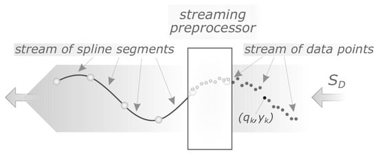
Figure 1. Conceptual diagram of the considered problem: the streaming preprocessor (segmenter) maps a stream of data points to a stream of cubic spline segments, which form a $C^2$-continuous curve.

The main contributions of this paper are the following:

• the cubic splinelet of type $WSS{R}_{min}$—the special type of splinelet that minimizes the Weighted Sum of Squared Residuals (Section 4.1),
• the algorithm for $C^2$-continuous $WSS{R}_{min}$-cubic splinelet-based adaptive segmentation of streaming sensor data (Section 4.2 and Section 4.3),
• numerical results which demonstrate the effectiveness of the algorithm (Section 5).

The remainder of this paper is organized as follows. The next Section 2 contains the related work overview. Following that Section 3, the problem statement is given and then, in Section 4, the proposed solution is described. Next Section 5, the solution is evaluated, and the obtained results are presented and discussed. The last Section 6 contains the conclusion of the study.

2. Related Work

Stream computing requires low-latency real-time algorithms that can process massive amounts of data generated by multiple sources at very high speed [4]. Such algorithms should be able to pre-process and analyze on-the-fly high-velocity streams of data coming from sources such as the Internet of Things (IoT) devices, sensor networks, wearable and mobile devices, market data.

The key value of data coming from such sources is their “freshness”, and they should be processed and analyzed as soon as they arrive, which is the key assumption of the big data stream analytics [4]. Such a requirement leads to the need for low-latency real-time algorithms because the batch computing approach, in which data should be stored first before it is processed and analyzed, is not sufficient [4,5,6]. In recent years, the research has mainly been focused on algorithms for real-time analysis of big data streams and there was not much research into the noisy or incomplete streaming data pre-processing phase [4].

Below, the research related to the proposed algorithm characteristic features—the real-time data stream segmentation, smoothing, and compression—is presented. Moreover, the related research works on splines are mentioned and the selected possible application areas for the proposed algorithm are reviewed.

2.1. Data Stream Segmentation

Sensors located in IoT devices generate data streams continuously. For some application areas, it is crucial to partition such data into segments to perform successful analysis using advanced algorithms, for example the machine learning ones.

Streaming segmentation of the signal realized on edge devices allows for:

• reconstruction of a sampled noisy signal (to maintain its continuity/smoothness class as a key feature (like non-negativity)) before the network transmission,
• signal compression (in experiments with test signals, we observed the data size reduction from 135 to 208 times, i.e., two orders of magnitude),
• reduction of network traffic (in the entire infrastructure),
• energy savings (in the entire infrastructure—the network communication is energy-intensive, and additionally the signal smoothed on edge devices no longer needs to be pre-processed in the cloud).

Recognition and prediction of human activities by real-time analysis of data streams coming from sensors and actuators is one of the areas of application of data stream segmentation [7]. The problem of automatic segmentation of data stream into activities in real time is a difficult one—there is no general approach for determining the end of the detected activity [7]. Sensor data stream segmentation has been the subject of many research works. Some proposed approaches were based on a time window with fixed length or on a dynamic time window including fixed number of events [8,9]. The other approaches were based on a real-time analysis of temporal information but either very intensive pre-processing was required, or the application was limited (for example to location analysis) [10,11].

An approach for continuous activity recognition based on the real-time sensor data segmentation was proposed in [12]. The proposed method was based on dynamically resized time windows (taking into account temporal sensor data and the state of activity recognition) and the ontology-based activity recognition algorithm. A real-time activity prediction method using automatic data stream segmentation based on Jaro–Winkler distance measurement was proposed in [7].

A method for unsupervised on-the-fly segmentation and classification of the time-series data was proposed in [13]. The approach was based on data density distribution estimation and the data stream was processed incrementally, using fixed amount of resources (memory and CPU). It even worked in real time when the sampling rate of the data stream was on the certain level [13]. A semantic-based approach for real-time separating and segmenting sensor data stream into multiple threads of activities was proposed in [14].

None of the above-mentioned approaches can provide online $C^2$-continuous segmentation. This is crucial if we must deal with physical constraints (for example, velocity and acceleration must be continuous).

Our proposed adaptive segmentation of the data stream (sampled signal) takes place in the approximation space of 3rd order splines (which represents the space of twice differentiable functions, i.e., the problem domain). Its result is a stream of segments that represents the reconstructed true signal. A spline constructed in this way recreates the signal taking into account its known class of continuity (smoothness). Therefore, we segment the data stream taking into account the features (continuity/smoothness class) of the processed signal.

2.2. Data Stream Smoothing

Advanced driving assistance systems and adaptive cruise control systems require high-accuracy, low-noise (or at least smoothed) data for proper functioning [15]. Data streams of estimated vehicle position can be obtained from different types of sensors: GPS, radar, LiDAR, gyroscopes, accelerometers, wheel speed sensors. Data coming from those sensors can be noisy and inaccurate due to many technical reasons. Such inaccuracies may lead to incorrect absolute positioning, unrealistic kinematics and inconsistent spacing between vehicles [15].

In car-following applications, the Kalman smoothing was used for improving the quality of data coming from one source (GPS) [16] or from multiple sensors [15,17]. The Kalman smoothing approach was also used for improving the vehicle positioning data coming from GPS and internal dead reckoning (gyroscopes, accelerometers, wheel speed) sensors [18].

The method for smoothing the data stream coming from ultrasonic sensors measuring the water level was proposed in [19]. The proposed approach included outlier detection using modified Z-scores based on the median absolute deviation and stream data smoothing based on the exponentially weighted moving average.

A relational database system was extended to include real-time method based on dynamic probabilistic models for filtering and smoothing data streams in [20]. In their approach, the authors used particle filters (a class of sequential Monte Carlo algorithms).

The data stream smoothing methods mentioned above do not include data stream segmentation nor compression. The approach using wavelet-based Kalman data smoothing for processing uncertain oil well-testing data, which included compression, was presented in [21]. However, the backward data smoothing was performed offline. The real-time approach proposed in this paper provides $C^2$-continuous segmentation and data smoothing.

Signals of $C^2$ continuity, recorded by sensors, constitute a substantial category/class (for example, recorded location of autonomous vehicles, drones or industrial robots). $C^2$ continuity (as a measure of smoothness) is a key characteristic of a signal (similar to, for example, monotonicity or non-negativity) and determines the problem domain. It means that the signal can be differentiated twice. For example, it allows, based on the recorded location of the object, the determination of its velocity and acceleration, without the need to additionally register these quantities which, in turn:

• significantly reduces the size of the data needed to be transferred from the edge layer to the cloud,
• reduces delays and speeds up data transmission,
• reduces energy consumption (in the entire infrastructure).

In the case of a noisy signal (a typical case), taking into account the continuity class allows for a more accurate reproduction of the true signal (noise removal). The continuity class is an important element of our knowledge about the signal, which we should not ignore because it reduces the accuracy of the true signal reproduction (the signal cannot represent, for example, the function of the object’s location in time, if it is not twice differentiable—otherwise it would allow the possibility of the operation of infinitely large forces, and we do not have such in nature).

2.3. Data Stream Compression

The cloud computing is an indispensable part of the Internet of Things (IoT). However, using it gives us many problems including transmission latency, bandwidth constraints, and high energy consumption [2]. Micro-controller, transceiver, and sensor units are the parts of smart devices that consume most of the energy, and data transmission is the most power-hungry task [22,23]. Energy efficiency can be improved by moving computation tasks from the cloud to edge devices, and by reducing the amount of data transferred from IoT devices to the edge (which additionally conserves the edge devices’ storage space) [1,2,24].

The proposed approaches for data reduction during transmission between IoT devices and edge computing devices were based on adaptive sampling [25,26,27], aggregation and compression [28,29,30,31,32], and Compressive Sensing [33,34,35,36]. The main disadvantage of the above approaches is the low compression ratio of non-stationary data coming from multiple sensors [2].

To address the above issue, in [2] a lightweight version of fast error-bounded lossy compression algorithm [37] was proposed. The authors showed that the proposed approach was able to reduce the amount of data transmitted from the wearable device to the edge device by approximately 103 times, simultaneously not worsening the results of data analytics.

None of the above-mentioned compression algorithms pre-process data into a form that would potentially accelerate the operation of machine learning algorithms on edge devices, for example by segmenting or smoothing the data stream before sending it from sensors or IoT devices.

Our algorithm segments the data stream (sampled signal belonging to the continuity class $C^2$) in an online way. Segmentation allows for a significant degree of compression (we have observed the data size reduction of 135 to 208 times) and the $C^2$ class of the signal helps in this process since three out of four coefficients of each spline segment (apart from the first one) can be calculated from the continuity conditions. The omission in the segmentation process of the known (in advance—because we know what we are measuring) continuity class of the processed signal could potentially allow for a slightly better compression ratio, but at the cost of the accuracy of signal reproduction (and in many cases it is unacceptable). It is primarily about recreating the qualitative characteristics of the signal (continuity/smoothness class), and less about the accuracy of approximation (quantitative feature, measured, for example, with the mean square error).

2.4. Splines

A spline—flexible strip of wood that was used to draw smooth curves—was mentioned for the first time in [38], as indicated in [39]. The new idea of a spline curve represented as piece-wise polynomial curves with certain smoothness properties was proposed in [40]. In this work, mathematical foundations for spline interpolation and approximation were presented. More information on splines can be found for example in the following works [41,42,43,44,45].

An approximation of a linearly varying curvature by three cubic curve segments was proposed in [46]. An online algorithm for the generation of minimum time joint industrial manipulators trajectories, using similar representation of a curve as in [46], was proposed in [47].

The real-time and online applications of interpolating splines were proposed in [48,49,50,51,52,53,54,55]. Among others, the application areas included trajectory generation and planning methods for robotic [53,54] and simulation-based sailboat trajectory optimization was [55].

To the best of our knowledge, there is no online algorithm, which can compute $C^2$-continuous segmentations. The approach proposed in this paper can perform online $C^2$-continuous cubic splinelet-based adaptive segmentation. It can process data streams in real time. It can also be applied offline when dealing with huge amounts of data, which cannot be processes by traditional algorithms due to memory limitations.

2.5. Possible Application Areas

The application areas, for which there is a need for on-the-fly algorithms allowing for data stream segmentation, smoothing, and compression include, but are not limited to, IoT devices, sensor networks, edge computing, and autonomous vehicles (cars, robots, drones). The need for real-time pre-processing of big data streams coming from multiple sensors results from data noise, bandwidth limitations and energy efficiency requirements. Below, the selected research in three areas (sensor networks, Unmanned Aerial Vehicles teams and robot teams), in which the proposed algorithm could be applied, is presented.

Weather prediction generally requires expensive weather stations and supercomputers for computations. An alternative can be the approach using Distributed Sensor Network for collecting data and performing weather prediction computations [56].

Such an approach requires real-time pre-processing, segmentation, smoothing, and compression of data streams because the used weather stations continuously communicate with each other and exchange large amounts of data coming from sensors to compute the predictions. The approach proposed in this paper meets all the requirements to be used in this area of applications—it allows for online $C^2$-continuous cubic splinelet-based adaptive segmentation, compression, and smoothing of noisy data streams.

Using multiple Unmanned Aerial Vehicles (UAVs) for surveillance, environmental monitoring, and rescue operations has become an increasingly popular research topic in the recent years [57,58]. Tracking single or multiple moving ground targets requires continuously updated and accurate data about their position. The accuracy of data coming from UAV’s sensors is crucial for that task. However, data coming from sensors such as GPS, radar, LiDAR, gyroscopes, and accelerometers can be noisy and inaccurate due to many technical reasons. Using multiple coordinated UAVs allows for combining data coming from their sensors and thus using more accurate information about the current target(s) position [57]. Furthermore, the navigation and coordination of the group of UAVs will require real-time continuous exchange of large amounts of data coming from each unit sensors [59].

Using a real-time algorithm that can segment, smooth and compress data streams coming from each UAV’s sensors will be crucial for successfully navigating and coordinating a whole team. The online algorithm proposed in this paper not only computes $C^2$-segmentations, but also smooths and compress data in real time, which makes it fully applicable in such a domain as UAVs’ sensors data analytics. The online $C^2$-continuous segmentation is crucial for UAVs because, for example, the approximated trajectory of a vehicle must be twice differentiable to give a continuous velocity and acceleration.

The research on multi-robot systems (MRS) gained importance and developed significantly in the recent years. Some of the most important research problems in MRS domain include communication mechanisms, planning and coordination strategies, and decision-making algorithms [60]. Research issues related to team coordination [61], sharing data, intelligence, and resources between many robots [62] are of great importance. The effective communication between many robots in the case of limited bandwidth resulting from environmental conditions (for example underwater environment), in which teams of robots are operating, is also the subject of intensive research [63]).

As in the case of drone teams, also in the case of robot teams coordinating their actions and sharing data, the essential issue is to deal in real time with data streams, which additionally can be noisy and incomplete. In such a case, using a method of segmenting, smoothing and compressing data in real time is crucial. The proposed approach not only does this, but also provides $C^2$-segmentations, which is of crucial importance when we use the data to plan the trajectories for robots. In such a case the trajectory must be twice differentiable to give a continuous velocity and acceleration.

3. Problem Formulation

Consider a stream of sensor data points, $S_D=\left(D_0,D_1,D_2,\dots \right)$, that arrive (or are accessed) sequentially, and describe an underlying signal $f\left(q\right)$, $q\in \mathbb{R}$ (note that in the subsequent formulae the q stands for any independent variable, typically it will refer to time (t)), where:

$$D_k=\left(q_k,f\left(q_k\right)\right)=\left(q_k,y_k\right).$$

(1)

This stream in a general case is “noisy”, i.e.,

$$f\left(q_k\right)=g\left(q_k\right)+{ϵ}_k,k=0,1,2\dots$$

(2)

where $g(·)$ is the true signal and $ϵ\sim \mathcal{N}(\mu ,{\sigma }^2)$, i.e., it is Gaussian noise. This model is shown in Figure 1.

Problem statement.

Given a stream of data points $S_D=\left(D_0,D_1,D_2,\dots \right)$, where $D_k=\left(q_k,y_k\right)$ with $y_k=g\left(q_k\right)+{ϵ}_k,k=0,1,2\dots$, find the $C^2$-continuous cubic spline whose segments correspond—in the space generated by the user-defined segment length adaptation strategy (δ)—to the optimal segmentation of $S_D$, with regard to the reconstruction of the original signal (g).

Remark 1.

The adaptation strategy, δ, usually depends on the target platform capabilities (e.g., the available memory), and on the required accuracy of the solution. In specific cases, it can be very sophisticated, e.g., Machine Learning (ML)-based.

4. Proposed Solution

The streaming algorithm we propose is based upon the concept of a cubic splinelet—a local building block of an “on the fly” constructed global cubic spline, which is by definition $C^2$-continuous (see Section 4.1 and [64]). This local, three-segment building block introduces a look-ahead capability to the algorithm, which—because of its online characteristic—must be greedy. Indeed, we can construct the global cubic spline using only the first segment of each splinelet, while the remaining two—treated as a “look-ahead” part—can be dropped (see Algorithm 1).

The key elements of the proposed algorithm (including its pseudo-code) are given in the following three subsections.

4.1. Cubic Splinelet of Type $WSS{R}_{min}$—The Solution Building Block

Without loss of generality, we can consider the problem in the following local frame:

$$(x,y)=(q-q_0,y)$$

(3)

which means that an interval $[q_A,q_D]$, given in the global frame, $Oqy$, is shifted in q-direction by the offset, $q_0$:

$$[q_A,q_D]\stackrel{\mathrm{shift}\mathrm{by}{q}_0}{\to }[x_A,x_D]=[q_A-q_0,q_D-q_0]$$

(4)

In a special case, when $q_0=q_A$, we get:

$$[q_A,q_D]\stackrel{\mathrm{shift}\mathrm{by}{q}_A}{\to }[x_A,x_D]=[0,q_D-q_A]$$

(5)

Note: this local frame, $Oxy$, will be used in the following paragraphs.

Definition 1.

A cubic splinelet of type $WSS{R}_{min}$ is a three-segment piece-wise cubic function defined in the local frame (when $q_0=q_A$) as ([64]):

$$s\left(x\right)=\left\{\begin{array}{cc}{s}^{\left(1\right)}\left(x\right)\hfill & 0\le x\le x_B\hfill \\ s^{\left(2\right)}\left(x\right)\hfill & x_B\le x\le x_C\hfill \\ s^{\left(3\right)}\left(x\right)\hfill & x_C\le x\le x_D\hfill \end{array}\right.$$

(6)

where:

$$s^{\left(i\right)}\left(x\right)=\sum _{j=1}^4{a}_j^{\left(i\right)}{x}^{4-j},i=1,2,3$$

(7)

and with the following properties:

• $s\left(x\right)$ is $C^2$-continuous on the interval $I_s=[0,x_D]$,
• $s\left(x\right)$ has the following boundary conditions:

  $$x_A=0:\left\{\begin{array}{c}s\left(x_A\right)=s_A\hfill \\ s^{\prime }\left(x_A\right)=s_A^{\prime }\hfill \\ s^{″}\left(x_A\right)=s_A^{″}\hfill \end{array}\right.$$

  (8)
• minimizes the Weighted Sum of Squared Residuals, i.e.,

  $$\mathrm{WSSR}=\sum _{i=1}^3\sum _{x_k\in I_s^{\left(i\right)}}{w}_i\left(x_k\right){\left[y_k-s^{\left(i\right)}\left(x_k\right)\right]}^2\to min$$

  (9)

  where: $I_s^{\left(1\right)}=[0,x_B)$, $I_s^{\left(2\right)}=[x_B,x_C)$ and $I_s^{\left(3\right)}=[x_C,x_D]$.

To find the splinelet corresponding to Equation (9), we first note that each coefficient in Equation (7) can be expressed in the following way:

$$a_j^{\left(i\right)}=A_{j1}^{\left(i\right)}{s}_D+A_{j2}^{\left(i\right)}{s}_D^{\prime }+A_{j3}^{\left(i\right)}{s}_D^{″}+A_{j4}^{\left(i\right)}=\sum _{l=1}^4{A}_{jl}^{\left(i\right)}{\alpha }_l$$

(10)

where: $i=1,2,3$, $j=1,2,3,4$, and $({\alpha }_1,{\alpha }_2,{\alpha }_3,{\alpha }_4)=(s_D,s_D^{\prime },s_D^{″},1)$. Equation (9) can be now restated as the following parametric optimization problem:

$$\mathrm{WSSR}=J({\alpha }_1,{\alpha }_2,{\alpha }_3)=\sum _{i=1}^3\sum _{x_k\in I_s^{\left(i\right)}}{w}_i\left(x_k\right){\left[y_k-\sum _{j=1}^4\sum _{l=1}^4{A}_{jl}^{\left(i\right)}{\alpha }_l{x}_k^{4-j}\right]}^2\to min$$

(11)

or, in another notation:

$$\underset{{\alpha }_1,{\alpha }_2,{\alpha }_3}{argmin}\sum _{i=1}^3\sum _{x_k\in I_s^{\left(i\right)}}{w}_i\left(x_k\right){\left[y_k-\sum _{j=1}^4\sum _{l=1}^4{A}_{jl}^{\left(i\right)}{\alpha }_l{x}_k^{4-j}\right]}^2.$$

(12)

Next, we compute:

$$\left\{\begin{array}{c}\frac{\partial J}{\partial {\alpha }_1}({\alpha }_1,{\alpha }_2,{\alpha }_3)=0\hfill \\ \frac{\partial J}{\partial {\alpha }_2}({\alpha }_1,{\alpha }_2,{\alpha }_3)=0\hfill \\ \frac{\partial J}{\partial {\alpha }_3}({\alpha }_1,{\alpha }_2,{\alpha }_3)=0\hfill \end{array}\right.$$

(13)

which leads to a system of three linear equations (since $J({\alpha }_1,{\alpha }_2,{\alpha }_3)$ is linear with respect to ${\alpha }_i$, $i=1,2,3$):

$$\sum _{j=1}^3{B}_{ij}{\alpha }_j=C_i,i=1,2,3$$

(14)

whose solution (i.e., the optimal values of ${\alpha }_i$, $i=1,2,3$) we substitute into Equation (10), and obtain the coefficients of the corresponding splinelet.

Remark 2.

Having set $w_i\left(x\right)$, $i=1,2,3$, and $x_A$, $x_B$, $x_C$, $x_D$, we can find the closed-form solution (compare [64]) for $a_j^{\left(i\right)}$, $i=1,2,3$, $j=1,2,3,4$.

4.2. Segmentation Heuristic Overview

The cubic splinelet defined in the previous section gives the locally optimal approximant in the given interval $[0,x_D]$. However, the following questions remain unanswered:

• What should be the value of $x_D$ that corresponds to the locally optimal stream segmentation/partitioning?
• What should be the search space for this optimization task?

The search space (interval) can be straightforwardly derived from the selected spline adaptation strategy. It may be as simple as:

$$Dom\left(x_D^{\left(i\right)}\right)=[x_{D_S}^{\left(i\right)},x_{D_E}^{\left(i\right)}]=[\frac{1}{2},2]x_D^{(i-1)}$$

(15)

The best $x_D$ can be then computed using an iterative improvement method. At each of its steps:

• the search interval is divided into predefined number of sub-intervals,
• they are then evaluated (see Equation (16) below) by sampling and interpolating (note: this step can be accelerated by memoization/caching),
• the best sub-interval becomes the new search interval.

The fitness (objective) function, $\varphi$, used in the above search algorithm is defined in the following way:

$$\varphi (s;\Delta R_{adj}^2,{\overline{L}}_1{}_{min},{\overline{L}}_1{}_{max})={\varphi }_1\left(s\right)+\Delta R_{adj}^2{\varphi }_2(s;{\overline{L}}_1{}_{min},{\overline{L}}_1{}_{max})$$

(16)

where:

$${\varphi }_1\left(s\right)=R_{adj}^2\left(s\right)=1-\frac{{\displaystyle \sum _{k=1}^n}{[y_k-s\left(x_k\right)]}^2}{{\displaystyle \sum _{k=1}^n}{(y_k-\overline{y})}^2}\frac{n-1}{n-4}$$

(17)

$${\varphi }_2(s;{\overline{L}}_1{}_{min},{\overline{L}}_1{}_{max})=\left\{\begin{array}{cc}\frac{{\overline{L}}_1{}_{max}-{\overline{L}}_1\left(s\right)}{{\overline{L}}_1{}_{max}-{\overline{L}}_1{}_{min}},\hfill & {\overline{L}}_1{}_{max}-{\overline{L}}_1{}_{min}>0\hfill \\ 1,\hfill & \mathrm{otherwise}\hfill \end{array}\right.$$

(18)

and:

$$\overline{y}=\frac{1}{n}\sum _{k=1}^n{y}_k$$

(19)

$$\Delta R_{adj}^2=\underset{s\in {\sum }_s}{max}{R}_{adj}^2\left(s\right)-\underset{s\in {\sum }_s}{min}{R}_{adj}^2\left(s\right)$$

(20)

$${\overline{L}}_1{}_{max}=\underset{s\in {\sum }_s}{max}\mathrm{MAE}\left(s\right)=\underset{s\in {\sum }_s}{max}\frac{1}{n}\sum _{k=1}^n|y_k-s\left(x_k\right)|$$

(21)

$${\overline{L}}_1{}_{min}=\underset{s\in {\sum }_s}{min}\mathrm{MAE}\left(s\right)=\underset{s\in {\sum }_s}{min}\frac{1}{n}\sum _{k=1}^n|y_k-s\left(x_k\right)|$$

(22)

with $R_{adj}^2$ being the Adjusted Coefficient of Determination, MAE—the Mean Absolute Error, and ${\sum }_s$—a set of candidate splinelets (corresponding to different values of $x_D$).

4.3. The Algorithm

Algorithm 1 presents a high-level view of the whole computational process (see also Appendix A). The sliding window-based streaming segmentation that we propose is clearly reflected in its structure. It is also worth noting that:

• the sliding window buffer size, h, can be either fixed upfront (e.g., depending on the input signal characteristics and/or real-time constraints), or constantly adapted (e.g., using ML algorithms); a good strategy for the first approach is to use the value of h corresponding to the maximum acceptable buffering delay (latency),
• to increase the readability of the pseudo-code, checking for exceptional/corner cases (e.g., too few data points at the end of the sliding window buffer to build one more segment) was omitted in some places,
• the algorithm presents one possible way of handling the end of the stream ($s_{Best}^{\left(3\right)}$, was computed with no looking-ahead); again, if necessary, this computation can be more sophisticated (e.g., the stream can be “artificially” extended),
• the number of sub-intervals that a given interval is divided into can be either fixed upfront or variable (e.g., simple dependence on the length of the interval, or ML-based).

Remark 3.

The streaming characteristic of the algorithm means that it requires $O\left(n\right)$ time and $O\left(h\right)$ space, where n stands for the length of ${\mathbf{S}}_{in}$ (potentially $n\to \infty$). See also Appendix B.

Algorithm 1. Adaptive segmentation of streaming data (see also Appendix A)

5. Results and Discussion

To evaluate the proposed algorithm, a series of numerical experiments was carried out, mostly in the form of a comparative analysis. As a point of reference, the results obtained from R function smooth.spline (accessed on 15 July 2021) were used. It is worth noting that this function—an example of state-of-the-art solutions—is global (i.e., the whole stream must be given as its input).

A summary of the evaluation process used is given in Section 5.1 and the results of the experiments are presented in Section 5.2 and Section 5.3.

5.1. Evaluation Process Overview

The key aspects of the evaluation process—test streams, algorithm performance descriptors, and the reference function (algorithm) used—are briefly described in this section.

5.1.1. Test Streams

The test data sets were generated using the following function g (its graph in the interval [0, 500] is shown in Figure 2) as the “true signal”:

$$g\left(q\right)=sin(\pi /2-0.1q)+sin\left(0.025q\right)+2sin\left(0.15q\right)$$

(23)

to which four levels of Gaussian noise was added, resulting in the following four test streams (see Figure 3):

$$\left\{\begin{array}{c}{f}_1\left(q_k\right)=g\left(q_k\right)+{ϵ}_{1_k}\hfill \\ f_2\left(q_k\right)=g\left(q_k\right)+{ϵ}_{2_k}\hfill \\ f_3\left(q_k\right)=g\left(q_k\right)+{ϵ}_{3_k}\hfill \\ f_4\left(q_k\right)=g\left(q_k\right)+{ϵ}_{4_k}\hfill \end{array}\right.$$

(24)

where:

$$q_k=0.05k,k=0,1,\dots ,{10}^6$$

(25)

$${ϵ}_{i_k}=\mathrm{first}\left[e|e\leftarrow \mathcal{N}(\mu =0,\sigma ={ϵ}_{i_{max}}/3),e<{ϵ}_{i_{max}}\right]$$

(26)

i.e., the first e, such that: $e\sim \mathcal{N}(\mu ,\sigma )$ and $e<{ϵ}_{i_{max}}$, and

$$[{ϵ}_{1_{max}},{ϵ}_{2_{max}},{ϵ}_{3_{max}},{ϵ}_{4_{max}}]=[0.1,0.5,1.5,3.5]$$

(27)

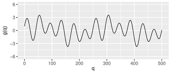
Figure 2. Signal g (Equation (2), for readability shown only in the interval $[0,500]$) used—after discretization and adding Gaussian noise—to generate the test streams used in the evaluation of the proposed algorithm.

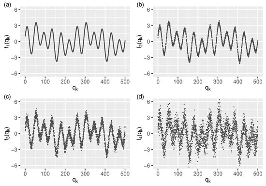
Figure 3. The test streams: (a–d) $f_1$–$f_4$ (for readability shown only in the interval $[0,500]$) generated from signal g using four levels of Gaussian noise (see Equation (27)).

5.1.2. Performance Descriptors

Each of the solutions, s, was evaluated using the following measures:

• Mean Absolute Error:

  $$\mathit{MAE}(s,f)=\frac{1}{n}\sum _{k=1}^n|s\left(x_k\right)-f\left(x_k\right)|$$

  (28)
• Root Mean Squared Error:

  $$\mathit{RMSE}(s,f)={\left\{\frac{1}{n}\sum _{k=1}^n{\left[s\left(x_k\right)-f\left(x_k\right)\right]}^2\right\}}^{1/2}$$

  (29)
• Normalized Root Squared Error:

  $$\mathit{NRSE}(s,f)={\left\{\frac{{\sum }_{k=1}^n{\left[s\left(x_k\right)-f\left(x_k\right)\right]}^2}{{\sum }_{k=1}^n{\left[f\left(x_k\right)\right]}^2}\right\}}^{1/2}$$

  (30)
• Mean Absolute Error Quotient (local-to-global algorithm ratio 1):

  $$Q_{\mathrm{MAE}}(s,s_R){|}_f=\frac{\mathit{MAE}(s,f)}{\mathit{MAE}(s_R,f)}$$

  (31)
• Root Mean Squared Error Quotient (local-to-global algorithm ratio 2):

  $$Q_{\mathrm{RMSE}}(s,s_R){|}_f=\frac{\mathrm{RMSE}(s,f)}{\mathit{RMSE}(s_R,f)}$$

  (32)
• Compression Ratio:

  $$\mathit{CR}(s,f)=\frac{\mathrm{uncompressed}\text{-}\mathrm{size}\left(f\right)}{\mathrm{compressed}\text{-}\mathrm{size}\left(f\right)}=\frac{\mathrm{size}\left(f\right)}{\mathrm{size}\left(s\right)}=\frac{\mathrm{length}\left({\mathbf{S}}_{in}\right)}{2+\mathrm{length}\left({\mathbf{S}}_{out}\right)}$$

  (33)
  Note: due to $C^2$-continuity of cubic splines we need only $\{4+[\mathrm{length}\left({\mathbf{S}}_{out}\right)-1]\}+\{\mathrm{length}\left({\mathbf{S}}_{out}\right)+1\}=2[2+\mathrm{length}\left({\mathbf{S}}_{out}\right)]$ values.
• Absolute Error (function):

  $$\mathit{AE}(x;s,f)=\left|s\right(x)-f(x\left)\right|$$

  (34)
• Squared Error (function):

  $$\mathit{SQE}(x;s,f)={\left[s\left(x\right)-f\left(x\right)\right]}^2$$

  (35)

Remark 4.

The above set covers local (AE and SQE), global (MAE, RMSE, and NRSE), and competitive ($Q_{\mathit{RMSE}}$, $Q_{\mathit{RMSE}}$, and CR) performance descriptors.

5.1.3. Reference Algorithm and Its Limitations

Remember that an online (local, streaming) algorithm is one that can process its input piece-by-piece in a serial fashion without having the entire input available from the beginning (as is the case for offline/global algorithms). As a result, it might make “decisions” that later turn out not to be optimal. Consequently, a local algorithm cannot outperform its global (optimal) counterpart. To compare these two, a “local-to-global algorithm ratio” is often used.

Unfortunately, this approach cannot be directly applied to the problem under consideration (i.e., adaptive segmentation of streaming data with the use of $C^2$-continuous cubic splines) because there is no other algorithm to compare it with. With this in mind, we can assume that the stream is finite and then use an existing cubic spline-based approximator as a (global) point of reference. An example of such an approximator is the R language smoothing spline function smooth.spline (accessed on 15 July 2021).

It turns out, however, that this is still not a solution because from the automatic segmentation point of view, this reference function (algorithm) does not handle data streams longer than about $6\%$ of the length of the test streams (as shown in Figure 4).

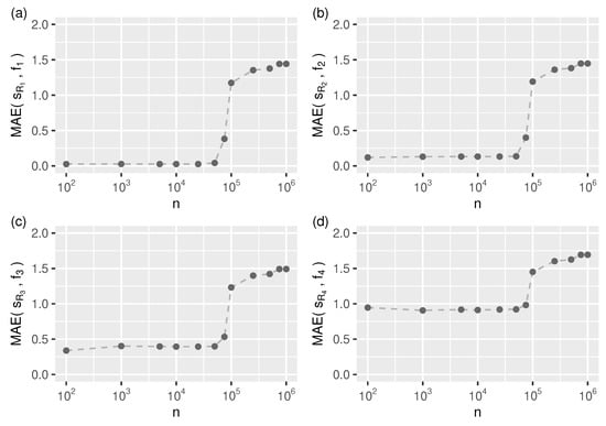
Figure 4. Auto-segmentation related limitations of the reference algorithm: approximation mean absolute error (Equation (28)) as a function of input stream length (n) for all test streams, (a–d) $f_1$–$f_4$. For $n>6\times {10}^4$ one needs to specify the number of spline segments (knots) manually.

For longer streams, we need to specify the number of smoothing spline segments (knots) manually. As shown in Figure 5, we can expect accurate approximations for all test streams when using more than $4\times {10}^3$ knots.

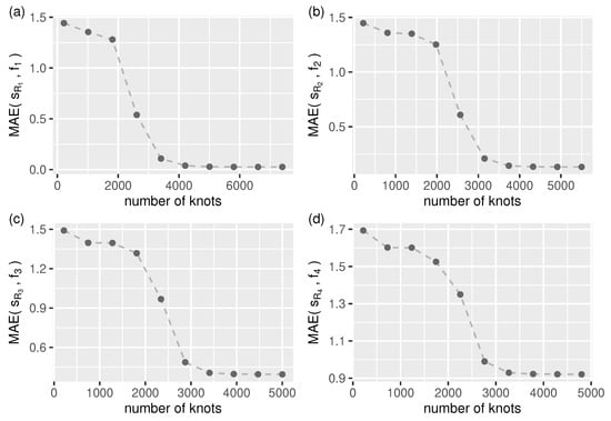
Figure 5. Approximation mean absolute error (Equation (28)) as a function of smooth.spline number of knots (segments) for all test streams, (a–d) $f_1$–$f_4$ (in all cases: $n={10}^6$).

Remark 5.

In the evaluation process used, the number of knots for function smooth.spline was set to be the same as that found by the splinelet-based segmentation algorithm (which in all cases was more than $4\times {10}^3$).

5.2. Evaluation Results: Approximation Errors and Compression Ratio

Given a signal, the quality of its splinelet-based approximation—measured in terms of absolute and quadratic errors (see Section 5.1.2)—is the key performance indicator of the corresponding segmentation which, in turn, is strongly related to the signal compression ratio. The corresponding evaluation results are presented in Table 1 and in Figure 5 and Figure 7.

Table 1. Performance comparative analysis (see Section 5.1.2): cubic splinelet generated spline (denoted as s) vs. smoothing spline (denoted as $s_R$) for all test streams $f_i$, where $i=1,2,3,4$.

f	MAE(s,f)	RMSE(s,f)	NRSE(s,f)	QMAE(s,${\mathit{s}}_{\mathit{R}}$)	QRMSE(s,${\mathit{s}}_{\mathit{R}}$)	CR(s,f)
$f_1$	0.029	0.037	0.021	1.110	1.243	135
$f_2$	0.136	0.170	0.098	1.033	1.070	183
$f_3$	0.402	0.502	0.279	1.019	1.040	201
$f_4$	0.933	1.165	0.560	1.013	1.028	208

The values of error quotients QMAE and QRMSE (Table 1) show that the splinelet-based solutions, despite being completely local, in most cases are almost as good as their global (smoothing spline-based) correspondents.

The same can be observed in Figure 6 and Figure 7. They provide additional insight into the splinelet-based approximation. These supplement the integral measure view—given by error quotients—with error distributions. Almost identical shapes of density lines corresponding to the two compared solutions confirm the high quality of splinelet-based solution. In this context, the values of compression ratios, $CR(s,t)$, given in Table 1 can be considered high (from 135 to 208, meaning that the compressed stream sizes are up to 208 times smaller).

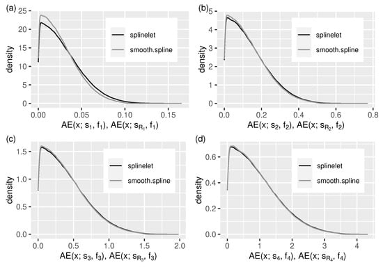
Figure 6. Cubic splinelet generated spline vs. smoothing spline: distribution of absolute approximation errors (in the form of a density function) for all test streams, (a–d) $f_1$–$f_4$.

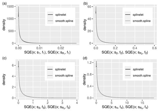
Figure 7. As in Figure 6, but for the squared approximation errors, $SQE$. (a–d) $f_1$–$f_4$.

5.3. Evaluation Results: Segment Length Auto-Adaptation

Since the spline segment length auto-adaptation mechanism determines the search space at each segmentation step, it has significant impact on the algorithm’s overall performance. Not only does this refer to the approximation quality (discussed in Section 5.2), but also—probably even more importantly—to the algorithm’s stability, which becomes essential in the context of the $C^2$-continuous streaming approximation.

Figure 8 shows concisely the spline segment auto-adaptation related results in the form of a segment length distribution for each tested data stream.

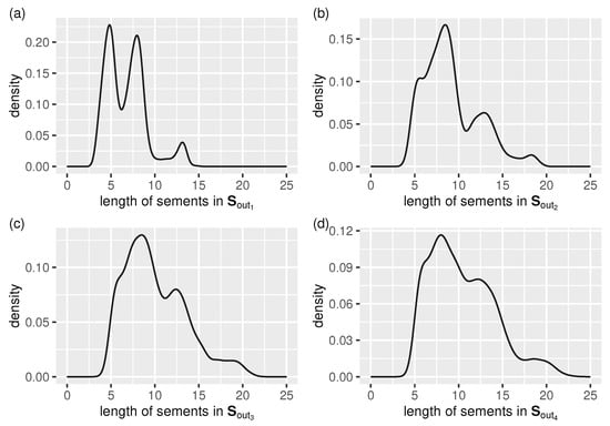
Figure 8. Output stream, ${\mathbf{S}}_{out}$, segment length auto-adaptation: distribution of cubic-splinelet-segment lengths (in the form of a density function) for all test streams, (a–d) $f_1$–$f_4$.

We can see that:

• in all cases the dominating segment lengths (remember that the test streams differ only in their signal-to-noise ratios—see Equations (23) and (26)) belong to the interval $[5,10]$,
• the lower the noise level, the more distinct the three existing maxima of the density function become (they correspond to the main “building blocks” used by the segmentation algorithm to restore the true signal, which is periodic),
• the higher the noise level, the closer to uniform the segment length distribution becomes, and the longer the segments are (because of a higher error tolerance).

Remark 6.

Although simple (see Equation (15)), the segment length auto-adaptation mechanism proved effective.

6. Conclusions

It has been shown that the $C^2$-continuous cubic splinelet-based adaptive segmentation of streaming data—despite its local/online character—is not only possible but also can be effective. The key element in achieving this was to base the algorithm on the greedy look-ahead strategy based on the concept of a cubic splinelet—a building block for $C^2$-continuous cubic splines. A characteristic feature of the proposed algorithm is the simultaneous segmentation, smoothing, and compression of data streams from sensors being performed in real time.

The segmentation quality has been measured in terms of the signal approximation accuracy and the corresponding compression ratio. The numerical results show the relatively high compression ratios (from 135 to 208, see Table 1) combined with the approximation errors comparable to these obtained from the (global) reference algorithm (see Figure 6 and Figure 7).

The proposed algorithm can be applied to various domains, including online compression and/or smoothing of streaming data coming from IoT devices, sensor networks, and sensors located in autonomous vehicles (cars, drones) and robots. The possible application areas also include real-time IoT analytics, and embedded time-series databases. Further exploration of this idea could be the first possible future research direction. Another could be related to more advanced auto-adaptation mechanisms of the search space.

References

- Shi, W.; Cao, J.; Zhang, Q.; Li, Y.; Xu, L. Edge Computing: Vision and Challenges. IEEE Internet Things J. 2016, 3, 637–646. [Google Scholar] [CrossRef]
- Azar, J.; Makhoul, A.; Barhamgi, M.; Couturier, R. An Energy Efficient IoT Data Compression Approach for Edge Machine Learning. Future Gener. Comput. Syst. 2019, 96, 168–175. [Google Scholar] [CrossRef]
- Papaioannou, T.G.; Riahi, M.; Aberer, K. Towards Online Multi-Model Approximation of Time Series. In Proceedings of the 2011 IEEE 12th International Conference on Mobile Data Management, Lulea, Sweden, 6–9 June 2011; pp. 33–38. [Google Scholar] [CrossRef]
- Kolajo, T.; Daramola, O.; Adebiyi, A. Big Data Stream Analysis: A Systematic Literature Review. J. Big Data 2019, 6, 47. [Google Scholar] [CrossRef]
- Qian, Z.; He, Y.; Su, C.; Wu, Z.; Zhu, H.; Zhang, T.; Zhou, L.; Yu, Y.; Zhang, Z. TimeStream: Reliable Stream Computation in the Cloud. In EuroSys’13: Proceedings of the 8th ACM European Conference on Computer Systems; ACM Press: Prague, Czech Republic, 2013; pp. 1–14. [Google Scholar] [CrossRef]
- Sun, D.; Zhang, G.; Zheng, W.; Li, K. Key Technologies for Big Data Stream Computing. In Big Data-Algorithms, Analytics, and Applications; Li, K., Jiang, H., Yang, L.T., Guzzocrea, A., Eds.; Chapman and Hall/CRC: New York, NY, USA, 2015; pp. 193–214. [Google Scholar] [CrossRef]
- Cho, H.; An, J.; Hong, I.; Lee, Y. Automatic Sensor Data Stream Segmentation for Real-Time Activity Prediction in Smart Spaces. In IoT-Sys’15: Proceedings of the 2015 Workshop on IoT Challenges in Mobile and Industrial Systems; Association for Computing Machinery: New York, NY, USA, 2015; pp. 13–18. [Google Scholar] [CrossRef]
- Laguna, J.O.; Olaya, A.G.; Borrajo, D. A Dynamic Sliding Window Approach for Activity Recognition. In User Modeling, Adaption and Personalization; Springer: Berlin/Heidelberg, Germany, 2011; pp. 219–230. [Google Scholar] [CrossRef]
- Tapia, E.M.; Intille, S.S.; Larson, K. Activity Recognition in the Home Using Simple and Ubiquitous Sensors. In Pervasive Computing; Springer: Berlin/Heidelberg, Germany, 2004; pp. 158–175. [Google Scholar] [CrossRef]
- Hong, X.; Nugent, C.D. Partitioning Time Series Sensor Data for Activity Recognition. In Proceedings of the 2009 9th International Conference on Information Technology and Applications in Biomedicine, Larnaka, Cyprus, 4–7 November 2009; pp. 1–4. [Google Scholar] [CrossRef]
- Wan, J.; O’Grady, M.J.; O’Hare, G.M.P. Dynamic Sensor Event Segmentation for Real-Time Activity Recognition in a Smart Home Context. Pers. Ubiquitous Comput. 2015, 19, 287–301. [Google Scholar] [CrossRef]
- Okeyo, G.; Chen, L.; Wang, H.; Sterritt, R. Dynamic Sensor Data Segmentation for Real-Time Knowledge-Driven Activity Recognition. Pervasive Mob. Comput. 2014, 10, 155–172. [Google Scholar] [CrossRef]
- Kohlmorgen, J.; Lemm, S. An On-Line Method for Segmentation and Identification of Non-Stationary Time Series. In Proceedings of the Neural Networks for Signal Processing XI: Proceedings of the 2001 IEEE Signal Processing Society Workshop (IEEE Cat, No. 01TH8584), North Falmouth, MA, USA, 12 September 2001; pp. 113–122. [Google Scholar] [CrossRef]
- Triboan, D.; Chen, L.; Chen, F.; Wang, Z. Semantic Segmentation of Real-Time Sensor Data Stream for Complex Activity Recognition. Pers. Ubiquitous Comput. 2017, 21, 411–425. [Google Scholar] [CrossRef]
- Bifulco, G.N. Real-Time Smoothing of Car-Following Data through Sensor-Fusion Techniques. Procedia Soc. Behav. Sci. 2011, 20, 524–535. [Google Scholar] [CrossRef][Green Version]
- Punzo, V.; Formisano, D.; Torrieri, V. Nonstationary Kalman Filter for Estimation of Accurate and Consistent Car-Following Data. Transp. Res. Rec. 2005, 1934, 2–12. [Google Scholar] [CrossRef]
- Ma, X.; Andreasson, I. Behavior Measurement, Analysis, and Regime Classification in Car Following. IEEE Trans. Intell. Transp. Syst. 2007, 8, 144–156. [Google Scholar] [CrossRef]
- Aono, T.; Fujii, K.; Hatsumoto, S.; Kamiya, T. Positioning of Vehicle on Undulating Ground Using GPS and Dead Reckoning. In Proceedings of the 1998 IEEE International Conference on Robotics and Automation (Cat, No.98CH36146), Leuven, Belgium, 20 May 1998; Volume 4, pp. 3443–3448. [Google Scholar] [CrossRef]
- Bae, I.; Ji, U. Outlier Detection and Smoothing Process for Water Level Data Measured by Ultrasonic Sensor in Stream Flows. Water 2019, 11, 951. [Google Scholar] [CrossRef]
- Kanagal, B.; Deshpande, A. Online Filtering, Smoothing and Probabilistic Modeling of Streaming Data. In Proceedings of the 2008 IEEE 24th International Conference on Data Engineering, Cancun, Mexico, 7–12 April 2008; pp. 1160–1169. [Google Scholar] [CrossRef]
- Feng, X.; Feng, Q.; Li, S.; Hou, X.; Zhang, M.; Liu, S. Wavelet-Based Kalman Smoothing Method for Uncertain Parameters Processing: Applications in Oil Well-Testing Data Denoising and Prediction. Sensors 2020, 20, 4541. [Google Scholar] [CrossRef]
- Anastasi, G.; Conti, M.; Di Francesco, M.; Passarella, A. Energy Conservation in Wireless Sensor Networks: A Survey. Ad Hoc Netw. 2009, 7, 537–568. [Google Scholar] [CrossRef]
- Razzaque, M.A.; Bleakley, C.; Dobson, S. Compression in Wireless Sensor Networks: A Survey and Comparative Evaluation. ACM Trans. Sens. Netw. 2013, 10, 1–44. [Google Scholar] [CrossRef]
- Miettinen, A.P.; Nurminen, J.K. Energy Efficiency of Mobile Clients in Cloud Computing. In HotCloud’10: Proceedings of the 2nd USENIX Conference on Hot Topics in Cloud Computing; USENIX Association: Berkeley, CA, USA, 2010; p. 4. [Google Scholar]
- Habib, C.; Makhoul, A.; Darazi, R.; Couturier, R. Real-Time Sampling Rate Adaptation Based on Continuous Risk Level Evaluation in Wireless Body Sensor Networks. In Proceedings of the 2017 IEEE 13th International Conference on Wireless and Mobile Computing, Networking and Communications (WiMob), Rome, Italy, 9–11 October 2017; pp. 1–8. [Google Scholar]
- Laiymani, D.; Makhoul, A. Adaptive Data Collection Approach for Periodic Sensor Networks. In Proceedings of the 2013 9th International Wireless Communications and Mobile Computing Conference (IWCMC), Sardinia, Italy, 1–5 July 2013; pp. 1448–1453. [Google Scholar]
- Tayeh, G.B.; Makhoul, A.; Laiymani, D.; Demerjian, J. A Distributed Real-Time Data Prediction and Adaptive Sensing Approach for Wireless Sensor Networks. Pervasive Mob. Comput. 2018, 49, 62–75. [Google Scholar] [CrossRef]
- Azar, J.; Makhoul, A.; Darazi, R.; Demerjian, J.; Couturier, R. On the Performance of Resource-Aware Compression Techniques for Vital Signs Data in Wireless Body Sensor Networks. In Proceedings of the 2018 IEEE Middle East and North Africa Communications Conference (MENACOMM), Jounieh, Lebanon, 18–20 April 2018; pp. 1–6. [Google Scholar]
- Alieksieiev, V. One Approach of Approximation for Incoming Data Stream in IoT Based Monitoring System. In Proceedings of the 2018 IEEE Second International Conference on Data Stream Mining & Processing (DSMP), Lviv, Ukraine, 21–25 August 2018; pp. 94–97. [Google Scholar]
- Azar, J.; Darazi, R.; Habib, C.; Makhoul, A.; Demerjian, J. Using DWT Lifting Scheme for Lossless Data Compression in Wireless Body Sensor Networks. In Proceedings of the 2018 14th International Wireless Communications & Mobile Computing Conference (IWCMC), Limassol, Cyprus, 25–29 June 2018; pp. 1465–1470. [Google Scholar]
- Harb, H.; Makhoul, A.; Abou Jaoude, C. En-Route Data Filtering Technique for Maximizing Wireless Sensor Network Lifetime. In Proceedings of the 2018 14th International Wireless Communications & Mobile Computing Conference (IWCMC), Limassol, Cyprus, 25–29 June 2018; pp. 298–303. [Google Scholar]
- Harb, H.; Makhoul, A.; Abou Jaoude, C. A Real-Time Massive Data Processing Technique for Densely Distributed Sensor Networks. IEEE Access 2018, 6, 56551–56561. [Google Scholar] [CrossRef]
- Cheng, L.; Guo, S.; Wang, Y.; Yang, Y. Lifting Wavelet Compression Based Data Aggregation in Big Data Wireless Sensor Networks. In Proceedings of the 2016 IEEE 22nd International Conference on Parallel and Distributed Systems (ICPADS), Wuhan, China, 13–16 December 2016; pp. 561–568. [Google Scholar] [CrossRef]
- Deligiannakis, A.; Kotidis, Y.; Roussopoulos, N. Compressing Historical Information in Sensor Networks. In SIGMOD’04: Proceedings of the 2004 ACM SIGMOD International Conference on Management of Data; ACM Press: Paris, France, 2004; p. 527. [Google Scholar] [CrossRef]
- Fragkiadakis, A.; Charalampidis, P.; Tragos, E. Adaptive Compressive Sensing for Energy Efficient Smart Objects in IoT Applications. In Proceedings of the 2014 4th International Conference on Wireless Communications, Vehicular Technology, Information Theory and Aerospace & Electronic Systems (VITAE), Aalborg, Denmark, 11–14 May 2014; pp. 1–5. [Google Scholar] [CrossRef]
- Gaeta, M.; Loia, V.; Tomasiello, S. Multisignal 1-D Compression by F-Transform for Wireless Sensor Networks Applications. Appl. Soft Comput. 2015, 30, 329–340. [Google Scholar] [CrossRef]
- Di, S.; Cappello, F. Fast Error-Bounded Lossy HPC Data Compression with SZ. In Proceedings of the 2016 IEEE International Parallel and Distributed Processing Symposium (IPDPS), Chicago, IL, USA, 23–27 May 2016; pp. 730–739. [Google Scholar]
- Monceau Du, H.L.D. Elémens de L’architecture Navale, ou Traité Pratique de la Construction des Vaisseaux; Chez Charles-Antoine Jombert: Paris, France, 1758. [Google Scholar]
- Farin, G.; Hoschek, J.; Kim, M.-S. Handbook of Computer Aided Geometric Design; Elsevier: Amsterdam, The Netherlands, 2002. [Google Scholar]
- Schoenberg, I. Contributions to the Problem of Approximation of Equidistant Data by Analytic Functions. Q. Appl. Math. 1946, 4, 45–99. [Google Scholar] [CrossRef]
- Boor de, C. A Practical Guide to Splines; Applied Mathematical Sciences; Springer: New York, NY, USA, 1978; Volume 27. [Google Scholar]
- Knott, G.D. Interpolating Cubic Splines; Progress in Computer Science and Applied Logic; Birkhäuser: Boston, MA, USA, 2000; Volume 18. [Google Scholar]
- Schoenberg, I.J. Cardinal Spline Interpolation; Siam: Philadelphia, PA, USA, 1973; Volume 12. [Google Scholar]
- Schumaker, L. Spline Functions: Basic Theory; Cambridge University Press: Cambridge, UK, 2007. [Google Scholar]
- Späth, H. One Dimensional Spline Interpolation Algorithms; A K Peters Series; CRC Press, Taylor & Francis Group: New York, NY, USA, 1995. [Google Scholar]
- Milenkovic, V.; Milenkovic, P.H. Tongue Model for Characterizing Vocal Tract Kinematics. In Recent Advances in Robot Kinematics; Springer: Dordrecht, The Netherlands, 1996; pp. 217–224. [Google Scholar]
- Bazaz, S.A.; Tondu, B. Minimum time on-line joint trajectory generator based on low order spline method for industrial manipulators. Robot. Auton. Syst. 1999, 29, 257–268. [Google Scholar] [CrossRef]
- Carvalho de, J.M.; Hanson, J.V. Real-time interpolation with cubic splines and polyphase networks. Can. Electr. Eng. J. 1986, 11, 64–72. [Google Scholar] [CrossRef]
- Fan, W.; Lee, C.H.; Chen, J.H. A realtime curvature-smooth interpolation scheme and motion planning for CNC machining of short line segments. Int. J. Mach. Tools Manuf. 2015, 96, 27–46. [Google Scholar] [CrossRef]
- Guven, O.; Eftekhar, A.; Kindt, W.; Constandinou, T.G. Computationally efficient real-time interpolation algorithm for non-uniform sampled biosignals. Healthc. Technol. Lett. 2016, 3, 105–110. [Google Scholar] [CrossRef]
- Ogniewski, J. Cubic Spline Interpolation in Real-Time Applications using Three Control Points. In Proceedings of the 27 International Conference in Central Europe on Computer Graphics, Visualization and Computer Vision WSCG 2019, Plzen, Czech Republic, 27–31 May 2019; World Society for Computer Graphics: Plzen, Czech Republic, 2019; pp. 1–10. [Google Scholar]
- Dębski, R. Real-time interpolation of streaming data. Comput. Sci. 2020, 21, 513–532. [Google Scholar] [CrossRef]
- Kröger, T. On-Line Trajectory Generation in Robotic Systems: Basic Concepts for Instantaneous Reactions to Unforeseen (Sensor) Events; Springer Tracts in Advanced Robotics; Springer: Berlin/Heidelberg, Germany, 2010; Volume 58. [Google Scholar]
- Biagiotti, L.; Melchiorri, C. Trajectory Planning for Automatic Machines and Robots; Springer: Berlin/Heidelberg, Germany, 2008. [Google Scholar]
- Dębski, R.; Sniezynski, B. Pruned Simulation-Based Optimal Sailboat Path Search Using Micro HPC Systems. In Computational Science–ICCS 2021, Lecture Notes in Computer Science; Paszynski, M., Kranzlmüller, D., Krzhizhanovskaya, V., Dongarra, J., Sloot, P., Eds.; Springer: Cham, Switzerland, 2021; Volume 12745, pp. 158–172. [Google Scholar] [CrossRef]
- Vas, Á.; Fazekas, Á.; Nagy, G.; Tóth, L. Distributed Sensor Network for Meteorological Observations and Numerical Weather Prediction Calculations. Carpathian J. Electron. Comput. Eng. 2013, 61, 56–63. [Google Scholar]
- Wise, R.; Rysdyk, R. UAV Coordination for Autonomous Target Tracking. In AIAA Guidance, Navigation, and Control Conference and Exhibit; American Institute of Aeronautics and Astronautics: Keystone, Colorado, 2006; pp. 1–22. [Google Scholar] [CrossRef]
- Chmaj, G.; Selvaraj, H. Distributed Processing Applications for UAV/Drones: A Survey. In Progress in Systems Engineering. Advances in Intelligent Systems and Computing; Selvaraj, H., Zydek, D., Chmaj, G., Eds.; Springer: Cham, Switzerland, 2015; Volume 366, pp. 449–454. [Google Scholar] [CrossRef]
- Huang, H.; Savkin, A.V.; Li, X. Reactive Autonomous Navigation of UAVs for Dynamic Sensing Coverage of Mobile Ground Targets. Sensors 2020, 20, 3720. [Google Scholar] [CrossRef] [PubMed]
- Yan, Z.; Jouandeau, N.; Ali, A. A Survey and Analysis of Multi-Robot Coordination. Int. J. Adv. Robot. Syst. 2013, 10, 399. [Google Scholar] [CrossRef]
- Almeida, L.; Santos, F.; Facchinetti, T.; Pedreiras, P.; Silva, V.; Lopes, L.S. Coordinating Distributed Autonomous Agents with a Real-Time Database: The CAMBADA Project. In Computer and Information Sciences-ISCIS 2004; Hutchison, D., Kanade, T., Kittler, J., Kleinberg, J.M., Mattern, F., Mitchell, J.C., Naor, M., Nierstrasz, O., Pandu Rangan, C., Steffen, B., et al., Eds.; Springer: Berlin/Heidelberg, Germany, 2004; Volume 3280, pp. 876–886. [Google Scholar] [CrossRef]
- López, D.S.; Moreno, G.; Cordero, J.; Sanchez, J.; Govindaraj, S.; Marques, M.M.; Lobo, V.; Fioravanti, S.; Grati, A.; Rudin, K.; et al. Interoperability in a Heterogeneous Team of Search and Rescue Robots. In Search and Rescue Robotics; IntechOpen: Rijeka, Croatia, 2017; Chapter 6; pp. 93–125. [Google Scholar] [CrossRef]
- Pfingsthorn, M.; Birk, A.; Bulow, H. An Efficient Strategy for Data Exchange in Multi-Robot Mapping under Underwater Communication Constraints. In Proceedings of the 2010 IEEE/RSJ International Conference on Intelligent Robots and Systems, Taipei, Taiwan, 18–22 October 2010; pp. 4886–4893. [Google Scholar] [CrossRef]
- Dębski, R. Streaming Hermite interpolation using cubic splinelets. Comput. Aided Geom. Des. 2021, 88, 102011. [Google Scholar] [CrossRef]
Publisher’s Note: MDPI stays neutral with regard to jurisdictional claims in published maps and institutional affiliations. |
© 2021 by the authors. Licensee MDPI, Basel, Switzerland. This article is an open access article distributed under the terms and conditions of the Creative Commons Attribution (CC BY) license (https://creativecommons.org/licenses/by/4.0/).