5.1. Simulation
Test 1. Protocol Efficiency
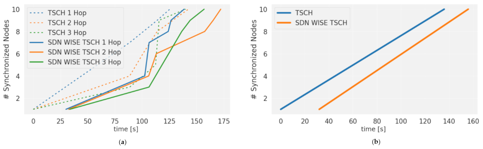
The network Convergence time depends mainly on the TSCH synchronization.
Figure 8a shows the result for a 1-s scan time on the four channels with one, two, and three hop networks. As can be seen, SDN convergence has a delay (continuous lines), because Topology Discovery starts after TSCH synchronization for each node. The increase in this time is not significant. According to
Figure 8b, the network takes 32 s more to be ready to send the first package.
The total Convergence time for SDN-WISE TSCH is given by TSCH’s Average Synchronization Time (
TS-TSCH) and Topology Discovery Time (
TTD) according to Equation (6)
The TSCH’s Average Synchronization Time is determined by Equation (7) according to [
42] multiplied by the number of hops (NH).
MT is the Average period for EB transmission, in our case 16 s. Taking into account that
C is the number of channels in TSCH schedule, 4 in the schedule used and the PDR is 1, by applying these values to Equation (7) a TS of 40 s is obtained. Considering that each node sends the information to the controller by the shortest route and taking into account the worst case, the most distant nodes, three hop routes would be used for the proposed topology, where
NH = 3. Thus, the total time for synchronization is equal to
TS-NH = 120 s, similar to that obtained in other works, see Figure 13 of [
43], where the Average Synchronization Time for 3 hops is around 155 s.
In addition, according to Equation (6), TTD must be considered, which in our case is around 32 s. With this, we finish with T ≈ TS · NH + TTD ≈ 120 s + 32 s ≈ 152 s approximately, which are the 152 s average obtained in the simulations.
After the convergence phase, it was observed that SDN-WISE continues to exchange messages and inform the controller of the topology on a regular basis. However, those protocols that make use of the RPL protocol are stabilized and exchange a smaller number of control packets [
12]. The number of packets generated by SDN-WISE is significantly higher than that of RPL,
Figure 9a. However, part of this difference is compensated by the byte size of the RPL packets, which is twice as large as the total number of bytes sent by each protocol, as shown in
Figure 9b. Although the number of bytes sent is still lower for the distributed protocol, most of these bytes are transmitted in the initial phase, while in SDN it is done constantly, so the initial peak in the RDC caused by TSCH synchronization will be increased; see
Figure 9c. The stability phase is still lower for SDN-WISE TSCH, because the controller has not configured any slots, while in distributed protocols, a certain number of slots per neighbor is automatically enabled, although it is not necessary.
The stability phase is still lower for SDN-WISE TSCH, because the controller is not set to any slot. The responsiveness of the controller to change the behavior of the WSN is the Configuration time. This is composed of two elements, the node arrival time and the scheduling processing and installation time, which is in charge of synchronizing packet generation. This last element is totally dependent on scheduling, while in distributed protocols, a certain number of slots per neighbor is automatically enabled, even though this is not necessary.
Figure 10 shows the sending of two OpenPathTSCH, one at timelot 0 and the other at timelot 590. For the first configuration packet, the node configures the sending frequency to 1 packet/slotframe. For the second packet, the previous schedule is changed and the sending frequency is changed to 2 packet/slotframe. Because OpenPathTSCH is transmitted on Shared Slot, the arrival time at the node is equivalent to the Shared End to End Delay (Shared_E2E). This time depends on the slotframe size, the number of hops to the destination node (NH), the number of shared slots, and the PDR. For a PDR of 100% according to Equation (8), we would have 38 timeslots. The new schedule is executed from the second active timeslot, since the first one is used to synchronize packet generation.
Test 2. Performance Evaluation
To evaluate the performance of SDN-WISE TSCH, a transmission was made over 42,000 timeslots for each of the flows of node 10. It was made with each one separately and the test was repeated with all the flows transmitting. In this way, it was possible to evaluate how the protocol adapts to the configured transmission frequencies without interfering with the other flows. Node 10 flows with 100 ms, 70 ms, and 200 ms deadlines were used. The scheduling algorithm used by SDN-WISE TSCH allows multiple transmission slots to be assigned to suit the needs of each flow. As obtained in the scheduling section, the optimal slot frame size for this case is 19 slots, where a total of 6 transmission slots are assigned to node 10. The slot frame size and number of transmission slots are configured so that the Packet inter-arrival time is always within the deadlines.
The result is shown in
Figure 11a, where the behavior is the same in the isolated and combined case. The flows behave in a totally deterministic way, according to the scheduling shown in
Figure 4. Flow 1 has two repetitions assigned and they are separated with 10 slots within the same slot frame and with 9 slots between slot frames. For this reason, two lines of the Packet inter-arrival time are shown. The same behavior shows flow 2 with 6 and 7 slots, and only flow 3 has a single value as it coincides with the size of the slot frame.
Figure 11b shows the different flows in the network, and the data flows have a completely linear growth, as they do not show any interruption. This is due to the fact that packet generation is synchronized with the slot frame, so each of the flows has the necessary resources assigned, avoiding losses and guaranteeing 100% DSR. For the case of the control flow, the initial part has a slow growth, since only the EB are exchanged. As the nodes are synchronized, there is a more noticeable increase in the flow, due to the introduction of the SDN-WISE TSCH control packages.
SDN-WISE TSCH maintains the transmission and reception characteristics in each of the flows regardless of whether they are isolated or combined. This is because, with the routes, TSCH scheduling, and packet marking, a slicing has been created that allows network resources to be allocated and conserved for each of the flows. In this way, there is no interference under normal conditions.
As has been observed so far, in this deployment of SDN-WISE TSCH, all information flows can be guaranteed so that neither excess control traffic nor other flows alter the scheduling of the network, thus obtaining high performance of the information flow.
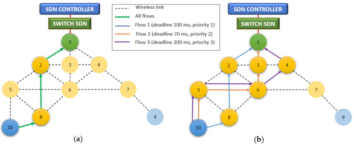
Figure 12a shows the advantages of using multiple paths. SDN-WISE TSCH differentiates flows by priority, which allows multiple paths to be assigned, distributing traffic over a larger number of nodes.
Figure 12b shows the use of the same path for all flows. This distribution has a direct impact on network performance and Network lifetime, as shown in
Figure 12c. The use of a single path generates a premature depletion of the central nodes. For the case of the single path, node 2 has the highest consumption and is 33% higher than the consumption of node 6, which is the highest consumption for the case of multipath. Although the general consumption in the case of multipath routes is 9% higher due to the greater number of hops, this consumption is not centered on a single node, it is distributed over a greater number of nodes, which allows the Network lifetime to be increased.
One of the advantages of distributed protocols is the ability to reconfigure autonomously, which allows the network to adapt to failures quickly. In a traditional SDN, this would require that the nodes instruct the controller to perform a reconfiguration. This would lead to a delay while the topology is recalculated, and the configuration is sent to the nodes. These delays and the excess of control traffic that occurs limit the use of centralized approaches, and for this reason in SDN WSN some decisions are left to the nodes. A system of states allows the nodes to alter the decisions of the controller based on local information. In this case, this possibility and the use of multiple routes is exploited to preserve the PDR of priority flows, redirecting the highest priority traffic when there is a failure.
Figure 13a shows the Packet inter-arrival time for node 10 during 7000 timeslots is kept constant while fulfilling the 100 and 70 ms deadline for flows 1 and 2. At 7500 timeslots, node 8 fails, and there is an increase in the Packet inter-arrival time of flow 1 of up to 40 timeslots. This is the time it takes for the buffer to exceed the configured occupancy limit, in this case, three packets. With the current generation period of flow 1 (10 timeslots), the limit is reached after 30 timeslots. The packet generated after reaching the limit is routed through the path assigned to flow 2. At this moment, the PDR is stabilized for flow 1
Figure 12b, in exchange for losing packets of lower priority from flow 2.
The peak that occurs in flow 2 is due to the controller reconfiguration time. After these 200 timeslots (2 s) the controller has sent a new schedule that meets the requirements set for each flow. The use of the state system, besides reducing the loss of packets by changing paths, allows the controller to be informed about the failure of node 8 immediately, thus skipping the time it takes the topology discovery to discover the failure, shortening the reconfiguration time to comparable levels of distributed protocols, as shown in
Figure 14 where a comparison has been made with Orchestra. When a failure occurs, in timeslot 4400, the packet inter arrival time increases to 250 timeslots for the distributed protocol as can be seen in
Figure 14a. However, for SDN-WISE it goes up only to 40 timeslots, while balancing the traffic of flow 1 and 2 on the second route. Thus, the packet loss is mitigated by the use of this route; see
Figure 14b. However, for the distributed protocol, it falls until the reconfiguration time is reached. For the case of SDN-WISE this time can be seen in the change of the End-to-End Delay of Flow 1; see
Figure 14c. When there is a failure the flow passes through the path of flow 2, so its End-to-End Delay is increased to the level defined for route 2, in this case, three timeslots. When the controller reconfigures the network, the flow returns to the End-to-End Delay of path with priority 1.
Test 3. Multiple Transmitters
The last parameter to be evaluated is the behavior of the network with additional traffic from other nodes. In this case, two flows from node 9.
Figure 15a shows the behavior of node 10, with a constant behavior up to 7600 timeslots, where the failure of node 8 occurs. Flow 1 is forwarded on path 2 and there is a packet loss (
Figure 15c), for flow 1 until it changes path and for flow 2 until the controller reconfigures. All this process generates additional control traffic that must be managed so that it does not affect other flows. In the case of node 9, the Packet Inter-arrival time for flow 1 of node 9 ranges from 7 to 12 timeslots (see
Figure 15b) because the algorithm has assigned two flows, one in slot 3 and another in slot 15. This configuration allows the deadline requirements to be met, and shows a cyclic behavior during the whole test, even in the moments when node 8 fails and node 10 requests a reconfiguration that increases the control traffic. No changes or alterations are seen in any of the flows. After these tests, it is verified that under normal conditions and alterations external to the node, a slice can be guaranteed for each flow and there is no interference between them, unless a network failure occurs, in which case the affected node will modify the packet sending to minimize the impact of the failure on the higher priority flow. The parameters measured in
Figure 15b show how there is no alteration in the flows of node 9, the PDR is maintained at 100%, and there is no unforeseen fluctuation in the Packet Inter-arrival Time.
In the tests shown in
Figure 15, flow 2 of node 9 was assigned a slot frame repeat, representing a Packet inter-arrival time of 190 ms. However, the deadline required for this flow is 300 ms, and meeting it by such a wide margin implies an excess of transmissions that can be avoided. For this reason, the scheduling algorithm chooses the size of the slot frame according to the flow with the highest deadline configured in the traffic descriptor.


 ,
, 


